ECE 493 - Probabilistic Reasoning and Decision Making
Review of Probability Theory 
Probability 
Definition
- Sample Space ($\Omega$): The set of all the outcomes of a random experiment.
- Event Space ($F$): A set whose elements $A \in F$ (called events) are subsets of $\Omega$.
Axioms of Probability
- $P(A) \ge 0, \forall A \in F$.
- $P(\cup_{i} A_{i}) = \sum_{i} P(A_{i})$ if $A_{1}, A_{2}, ...$ are disjoint events.
- $P(\Omega) = 1$.
Properties of Probability
- $A \subseteq B \implies P(A) \le P(B)$.
- $P(A \cap B) \le \min(P(A), P(B))$.
- Union Bound: $P(A \cup B) \le P(A) + P(B)$.
- Complement: $P(\Omega - A) = 1 - P(A)$.
- Law of Total Probability: $\sum_{i = 1}^{k} P(A_{i}) = 1$ if $A_{1}, ..., A_{k}$ are disjoint events and $\cup_{i = 1}^{k} A_{i} = \Omega$.
Conditional Probability
- The conditional probability of $A$, conditioned on $B$, is the probability that $A$ occurs given that $B$ has definitely occured. $$ \begin{aligned} P(A \mid B) &= \frac{P(A \cap B)}{P(B)} \\ &= \frac{P(B \mid A) \cdot P(A)}{P(B)} \end{aligned} $$
Chain Rule
- Let $S_{1}, ..., S_{k}$ be events, $P(S_{i}) > 0$. $$ \begin{aligned} & P(S_{1} \cap S_{2} \cap \cdots \cap S_{k}) \\ &= P(S_{1}) P(S_{2} \mid S_{1}) P(S_{3} \mid S_{2} \cap S_{1}) \cdots P(S_{k} \mid S_{1} \cap S_{2} \cap \cdots \cap S_{k - 1}) \end{aligned} $$
- If $k = 2$, $$P(S_{1} \cap S_{2}) = P(S_{1}) P(S_{2} \mid S_{1})$$
Independence
- Two events $A$ and $B$ are independent if and only if $$ \begin{aligned} P(A \cap B) &= P(A) P(B) \\ P(A \vert B) &= P(A) \\ P(B \vert A) &= P(B) \end{aligned} $$
Pairwise Independence
- Events $A_{1}, ..., A_{k}$ are pairwise independent if each pair is independent.
Conditional Independence
- Events $A_{1}, ..., A_{k}$ are conditionally independent conditioned on event $B$ if $$P(A_{1} \cap ... \cap A_{k} \mid B) = P(A_{1} \mid B) ... P(A_{k} \mid B)$$
Random Variables 
Definition
- A random variable $X$ is a function $X : \Omega \to \mathbb{R}$.
Cumulative Distribution Functions
- A cumulative distribution function (CDF) is a function $F_{X} : \mathbb{R} \to [0, 1]$ such that $F_{X}(x) = P(X \le x)$.
Properties of Cumulative Distribution Functions
- $0 \le F_{X}(x) \le 1$.
- $\lim_{x \to -\infty} F_{X}(x) = 0$.
- $\lim_{x \to +\infty} F_{X}(x) = 1$.
- $x \le y \implies F_{X}(x) \le F_{X}(y)$.
Probability Mass Functions (Discrete)
- A probability mass function (PMF) is a function $p_{X} : \Omega \to \mathbb{R}$ such that $p_{X}(x) = P(X = x)$.
Properties of Probability Mass Functions
- $0 \le p_{X}(x) \le 1$.
- $\sum_{x \in \text{Values}(X)} p_{X}(x) = 1$.
- $\sum_{x \in A} p_{X}(x) = P(X \in A)$.
Probability Density Functions (Continuous)
- A probability density function (PDF) is a function $f_{X}(x) : \Omega \to \mathbb{R}$ such that $f_{X}(x) = \frac{dF_{X}(x)}{dx}$.
Properties of Probability Density Functions
- $f_{X}(x) \ge 0$.
- $\int_{-\infty}^{\infty} f_{X}(x) = 1$.
- $\int_{x \in A} f_{X}(x) dx = P(X \in A)$.
Expectation
- Suppose that $X$ is a discrete random variable with PMF $p_{X}(x)$ and $g : \mathbb{R} \to \mathbb{R}$ is an arbitrary function. The expected value of $g(X)$ is the following. $$\mathbb{E}[g(X)] = \sum_{x \in \text{Values}(X)} g(x) p_{X}(x)$$
- Suppose that $X$ is a continuous random variable with PDF $f_{X}(x)$ and $g : \mathbb{R} \to \mathbb{R}$ is an arbitrary function. The expected value of $g(X)$ is the following. $$\mathbb{E}[g(X)] = \int_{-\infty}^{\infty} g(x) f_{X}(x) dx$$
Properties of Expectation
- $\mathbb{E}[a] = a$ for any constant $a \in \mathbb{R}$.
- $\mathbb{E}[a \cdot f(X)] = a \cdot \mathbb{E}[f(X)]$ for any constant $a \in \mathbb{R}$.
- $\mathbb{E}[f(X) + g(X)] = \mathbb{E}[f(X)] + \mathbb{E}[g(X)]$.
Variance
- The variance of a random variable $X$ is a measure of how concentrated the distribution of a random variable $X$ is around its mean. $$ \begin{aligned} \text{Var}[X] &= \mathbb{E}[(X - \mathbb{E}[X])^{2}] \\ &= \mathbb{E}[X^{2}] - \mathbb{E}[X]^{2} \end{aligned} $$
Properties of Variance
- $\text{Var}[a] = 0$ for any constant $a \in \mathbb{R}$.
- $\text{Var}[a \cdot f(x)] = a^{2} \cdot \text{Var}[f(x)]$ for any constant $a \in \mathbb{R}$.
Two Random Variables 
Joint and Marginal Distributions
- The joint cumulative distribution function of $X$ and $Y$ is defined by the following. $$F_{XY}(x, y) = P(X \le x, Y \le y)$$
- The marginal cumulative distribution functions of $F_{XY}(x, y)$ is defined by the following. $$ \begin{aligned} F_{X}(x) &= \lim_{y \to \infty} F_{XY}(x, y) \\ F_{Y}(y) &= \lim_{x \to \infty} F_{XY}(x, y) \end{aligned} $$
Properties of Joint Distributions
- $0 \le F_{XY}(x, y) \le 1$.
- $\lim_{x,y \to \infty} F_{XY}(x, y) = 1$.
- $\lim_{x,y \to -\infty} F_{XY}(x, y) = 0$.
Joint and Marginal Probability Mass Functions
- If $X$ and $Y$ are discrete random variables, then the joint probability mass function $p_{XY} : \text{Values}(X) \times \text{Values}(Y) \to [0, 1]$ is defined by the following. $$p_{XY}(x, y) = P(X = x, Y = y)$$
- The marginal probability mass functions of $p_{XY}$ are defined by the following. $$ \begin{aligned} p_{X}(x) &= \sum_{y} p_{XY}(x, y) \\ p_{Y}(y) &= \sum_{x} p_{XY}(x, y) \end{aligned} $$
Joint and Marginal Probability Density Functions
- If $X$ and $Y$ are continuous random variables, then the joint probability density function $f_{XY} : \text{Values}(X) \times \text{Values}(Y) \to \mathbb{R}$ is defined by the following. $$f_{XY}(x, y) = \frac{\partial^{2} F_{XY}(x, y)}{\partial x \partial y}$$
- The marginal probability density functions of $f_{XY}$ are defined by the following. $$ \begin{aligned} f_{X}(x) &= \int_{-\infty}^{\infty} f_{XY}(x, y) dy\\ f_{Y}(y) &= \int_{-\infty}^{\infty} f_{XY}(x, y) dx \end{aligned} $$
Conditional Distributions
- The conditional probability mass function of $Y$ given $X$ is defined by the following. $$p_{Y \mid X}(y \mid x) = \frac{p_{XY}(x, y)}{p_{X}(x)}$$
- The conditional probability density function of $Y$ given $X$ is defined by the following. $$f_{Y \mid X}(y \mid x) = \frac{f_{XY}(x, y)}{f_{X}(x)}$$
Chain Rule
$$ \begin{aligned} & p_{X_{1}, ..., X_{n}}(x_{1}, ..., x_{n}) \\ &= p_{X_{1}}(x_{1}) p_{X_{2} \mid X_{1}}(x_{2} \mid x_{1}) ... p_{X_{n} \mid X_{1}, ..., X_{n - 1}}(x_{n} \mid x_{1}, ..., x_{n - 1}) \end{aligned} $$Bayes' Rule
- For discrete random variables $X$ and $Y$, $$P_{Y \mid X}(y \mid x) = \frac{P_{XY}(x, y)}{P_{X}(x)} = \frac{P_{X \mid Y}(x \mid y) P_{Y}(y)}{\sum_{y' \in \text{Values}(Y) P_{X \mid Y}(x \mid y') P_{Y}(y')}}$$
- For continuous random variables $X$ and $Y$, $$f_{Y \mid X}(y \mid x) = \frac{f_{XY}(x, y)}{f_{X}(x)} = \frac{f_{X \mid Y}(x \mid y) f_{Y}(y)}{\int_{-\infty}^{\infty} f_{X \mid Y}(x \mid y') f_Y(y') dy'}$$
Independence
- For discrete random variables, $p_{XY}(x, y) = p_{X}(x) p_{Y}(y)$ for all $x \in \text{Values}(X)$, $y \in \text{Values}(Y)$.
- For discrete random variables, $p_{Y \mid X}(y \mid x) = p_{Y}(y)$ whenever $p_{X}(x) \ne 0$ for all $y \in \text{Values}(Y)$.
- For continuous random variables, $f_{XY}(x, y) = f_{X}(x) f_{Y}(y)$ for all $x \in \mathbb{R}$, $y \in \mathbb{R}$.
- For continuous random variables, $f_{Y \mid X}(y \mid x) = f_{Y}(y)$ whenever $f_{X}(x) \ne 0$ for all $y \in \mathbb{R}$.
Independence Lemma
- If $X$ and $Y$ are independent, then for any subsets $A, B \subseteq \mathbb{R}$, $$P(X \in A, Y \in B) = P(X \in A) P(Y \in B)$$
Expectation and Covariance
- Suppose that $X$ and $Y$ are random variables, and $g : \mathbb{R}^{2} \to \mathbb{R}$ is a function of these two random variables. The expected value of $g(X, Y)$ is the following. $$ \begin{aligned} \mathbb{E}[g(X,Y)] &= \sum_{x \in \text{Values}(X)} \sum_{y \in \text{Values}(Y)} g(x, y) p_{XY}(x, y) \\ \mathbb{E}[g(X,Y)] &= \int_{-\infty}^{\infty} \int_{-\infty}^{\infty} g(x, y) f_{XY}(x, y) dx dy \end{aligned} $$
- The covariance of two random variables $X$ and $Y$ is defined by the following. $$ \begin{aligned} \text{Cov}[X, Y] &= \mathbb{E}[(X - \mathbb{E}[X])(Y - \mathbb{E}[Y])] \\ &= \mathbb{E}[XY] - \mathbb{E}[X] \mathbb{E}[Y] \end{aligned} $$
Properties of Expectation and Covariance
- $\mathbb{E}[f(X, Y) + g(X,Y)] = \mathbb{E}[f(X, Y)] + \mathbb{E}[g(X, Y)]$.
- $\text{Var}[X + Y] = \text{Var}[X] + \text{Var}[Y] + 2\text{Cov}[X, Y]$.
- If $X$ and $Y$ are independent, then $\text{Cov}[X, Y] = 0$.
- If $X$ and $Y$ are independent, then $\mathbb{E}[f(X)g(Y)] = \mathbb{E}[f(X)] \mathbb{E}[g(Y)]$.
Representation 
- Problem: How do we express a probability distribution $p(x_{1}, x_{2}, ..., x_{n})$ that models some real-world phenomenon?
- Naive Complexity: $O(d^{n})$
- Solution: Representation with Probabilistic Graphical Models + Verifying Independence Assumptions
Bayesian Networks (Directed Probabilistic Graphical Model) 
Definition - What is a Bayesian network?
- A Bayesian network is a directed graph $G$ with the following:
- Nodes: A random variable $x_{i}$.
- Edges: A conditional probability distribution (CPD) $p(x_{i} \mid x_{A_{i}})$ per node, specifying the probability of $x_i$ conditioned on its parent's values.
Representation - How does a Bayesian network express a probability distribution?
- Let $p$ be a probability distribution.
- A naive representation of $p$ can be derived using the chain rule: $$p(x_{1}, x_{2}, ..., x_{n}) = p(x_{1}) p(x_{2} \mid x_{1}) \cdots p(x_{n} \mid x_{n - 1}, ..., x_{2}, x_{1})$$
- A Bayesian network representation of $p$ compacts the naive representation by having each factor in the right hand side depend only on a small number of ancestor variables $x_{A_{i}}$:
$$p(x_{i} \mid x_{i - 1}, ..., x_{2}, x_{1}) = p(x_{i} \mid x_{A_{i}})$$
- e.g., Approximate $p(x_{5} \mid x_{4}, x_{3}, x_{2}, x_{1})$ with $p(x_{5} \mid x_{A_{5}})$ where $x_{A_{5}} = \{x_{4}, x_{3}\}$.
Space Complexity - How compact is a Bayesian network?
- Consider each of the factors $p(x_{i} \mid x_{A_{i}})$ as a probability table:
- Rows: Values of $x_{i}$
- Columns: Values of $x_{A_{i}}$
- Cells: Values of $p(x_{i} \mid x_{A_{i}})$
- If each discrete random variable takes $d$ possible values and has at most $k$ ancestors, then each probability table has at most $O(d^{k + 1})$ entries.
- Naive Representation Space Complexity: $O(d^n)$
- Bayesian Networks Representation Space Complexity: $O(n \cdot d^{k + 1})$ $$\approx \text{Bayesian Networks Representation} \le \text{Naive Representation}$$
Independence Assumptions - Why are the independence assumptions of a Bayesian network important to identify?
- A Bayesian network expresses a probability distribution $p$ via products of smaller, local conditional probability distributions (one for each variable).
- These smaller, local conditional probability distributions introduces assumptions into the model of $p$ that certain variables are independent.
- Important Note: Which independence assumptions are we exactly making by using a Bayesian network?
- Correctness: Are these independence assumptions correct?
- Efficiency: Do these independence assumptions efficiently compact the representation?
$3$-Variable Independencies in Directed Graphs - How do you identify independent variables in a $3$-variable Bayesian network?
- Let $x \perp y$ indicate that variables $x$ and $y$ are independent.
- Let $G$ be a Bayesian network with three nodes: $A$, $B$, and $C$.
Common Parent
- If $G$ is of the form $A \leftarrow B \rightarrow C$,
- If $B$ is observed, then $A \perp C \mid B$
- If $B$ is unobserved, then $A \not\perp C$
- Intuition: $B$ contains all the information that determines the outcomes of $A$ and $C$; once it is observed, there is nothing else that affects $A$'s and $C$s' outcomes.
Cascade
- If $G$ equals $A \rightarrow B \rightarrow C$,
- If $B$ is observed, then $A \perp C \mid B$
- If $B$ is unobserved, then $A \not\perp C$
- Intuition: $B$ contains all the information that determines the outcomes of $C$; once it is observed, there is nothing else that affects $C$'s outcomes.
V-Structure
- If $G$ is $A \rightarrow C \leftarrow B$, then knowing $C$ couples $A$ and $B$.
- If $C$ is unobserved, then $A \perp B$
- If $C$ is observed, then $A \not\perp B \mid C$
$n$-Variable Independencies in Directed Graphs - How do you identify independent variables in a $n$-variable Bayesian network?
- Let $I(p)$ be the set of all independencies that hold for a probability distribution $p$.
- Let $I(G) = \{(X \perp Y \mid Z) : X, Y \text{ are } d\text{-sep given } Z\}$ be a set of variables that are $d$-separated in $G$.
- If the probability distribution $p$ factorizes over $G$, then $I(G) \subseteq I(p)$ and $G$ is an $I$-map (independence map) for $p$.
- Important Note 1: Thus, variables that are $d$-separated in $G$ are independent in $p$.
- Important Note 2: However, a probability distribution $q$ can factorize over $G$, yet have independencies that are not captured in $G$.
- Important Caveat: A Bayesian network cannot perfectly represent all probability distributions.
$d$-separation (a.k.a. Directed Separation)
- $Q$ and $W$ are $d$-separated when variables $O$ are observed if they are NOT CONNECTED by an active path.
Active Path
- An undirected path in the Bayesian Network structure $G$ is called active given observed variables $O$ if for EVERY CONSECUTIVE TRIPLE of variables $X$, $Y$, $Z$ on the path, one of the following holds:
- Evidential Trail: $X \leftarrow Y \leftarrow Z$, and $Y$ is unobserved $Y \not\in O$
- Causal Trail: $X \rightarrow Y \rightarrow Z$, and $Y$ is unobserved $Y \not\in O$
- Common Cause: $X \leftarrow Y \rightarrow Z$, and $Y$ is unobserved $Y \not\in O$
- Common Effect: $X \rightarrow Y \leftarrow Z$, and $Y$ or any of its descendants are observed
Equivalence - When are two Bayesian networks $I$-equivalent?
- $G_1$ and $G_2$ are $I$-equivalent...
- If they encode the same dependencies: $I(G_1) = I(G_2)$.
- If they have the same skeleton and the same v-structures.
- If the $d$-separation between variables is the same.
Skeleton
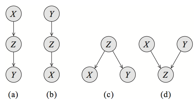
- A skeleton is an undirected graph obtained by dropping the directionality of the arrows.
- (a) is Cascade
- (b) is Cascade
- (c) is Common Parent
- (d) is V-Structure
- (a), (b), (c), and (d) have the same skeleton.
Example Problem 1 - $d$-separation
Question
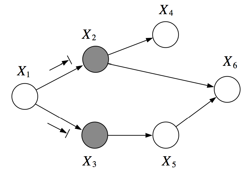
- Are $X_{1}$ and $X_{6}$ $d$-separated given $\{X_{2}, X_{3}\}$?
Solution
- Path: $X_{1} \rightarrow X_{2} \rightarrow X_{6}$
- Consecutive Triple: $X_{1} \rightarrow X_{2} \rightarrow X_{6}$
- Although $X_{2}$ is observed, the common effect does not hold.
- As not all the consecutive triples hold, this path is not active.
- Consecutive Triple: $X_{1} \rightarrow X_{2} \rightarrow X_{6}$
- Path: $X_{1} \rightarrow X_{3} \rightarrow X_{5} \rightarrow X_{6}$
- Consecutive Triple: $X_{1} \rightarrow X_{3} \rightarrow X_{5}$
- Although $X_{3}$ is observed, the common effect does not hold.
- Consecutive Triple: $X_{3} \rightarrow X_{5} \rightarrow X_{6}$
- As $X_{5}$ is unobserved, the causal trail does hold.
- As not all the consecutive triples hold, this path is not active.
- Consecutive Triple: $X_{1} \rightarrow X_{3} \rightarrow X_{5}$
- As there are no active paths between $X_{1}$ and $X_{6}$, they are $d$-separated given $\{X_{2}, X_{3}\}$.
Example Problem 2 - $d$-separation
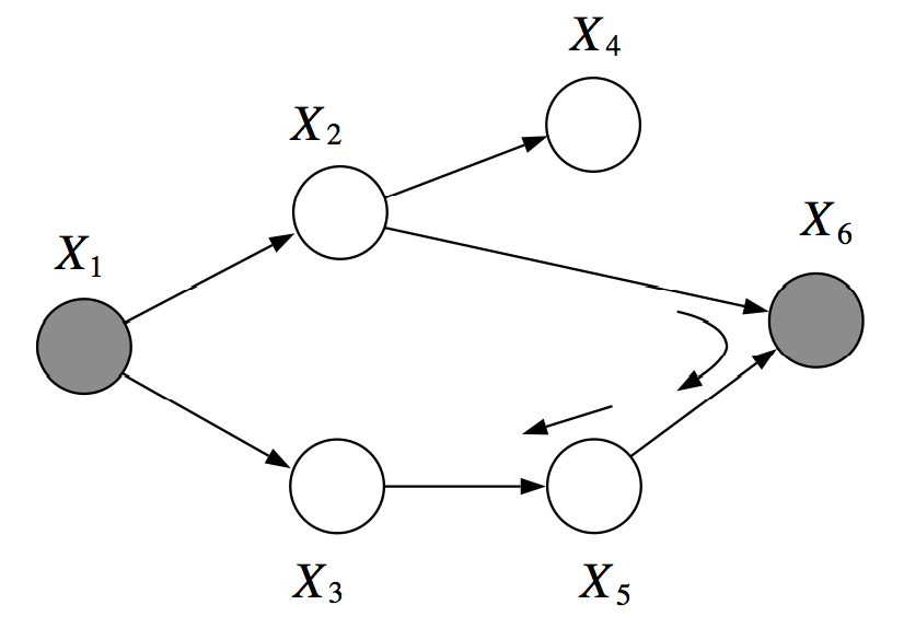
Question
- Are $X_{2}$ and $X_{3}$ $d$-separated given $\{X_{1}, X_{6}\}$?
Solution
- Path: $X_{2} \leftarrow X_{1} \rightarrow X_{3}$
- Consecutive Triple: $X_{2} \leftarrow X_{1} \rightarrow X_{3}$
- Although $X_{1}$ is observed, the common effect does not hold.
- As not all the consecutive triples hold, this path is not active.
- Consecutive Triple: $X_{2} \leftarrow X_{1} \rightarrow X_{3}$
- Path: $X_{2} \rightarrow X_{6} \leftarrow X_{5} \leftarrow X_{3}$
- Consecutive Triple: $X_{2} \rightarrow X_{6} \leftarrow X_{5}$
- As $X_{6}$ is observed, the common effect does hold.
- Consecutive Triple: $X_{6} \leftarrow X_{5} \leftarrow X_{3}$
- As $X_{5}$ is unobserved. the causal trail does hold.
- As all the consecutive triples hold, this path is active.
- Consecutive Triple: $X_{2} \rightarrow X_{6} \leftarrow X_{5}$
- As there exists an active path between $X_{2}$ and $X_{3}$, they are not $d$-separated given $\{X_{1}, X_{6}\}$.
Markov Random Fields (Undirected Probabilistic Graphical Model) 
Definition - What is a Markov random field?
- A Markov random field is an undirected graph $G$ with the following:
- Nodes: A random variable $x_{i}$.
- Fully Connected Subgraphs: An optional factor $\phi_{c}(x_{c})$ per clique, specifying the level of coupling (potentials) between all the dependent variables within the clique.
- Important Note:
...SPECIFYING THE LEVEL OF COUPLING BETWEEN ALL THE DEPENDENT VARIABLES WITHIN THE CLIQUE...
Representation - How does a Markov random field express a probability distribution?
- Let $p$ be a probability distribution.
- A Markov random field representation of $p$ is the following:
$$p(x_{1}, x_{2}, ..., x_{n}) = \frac{1}{Z} \prod_{c \in C} \phi_{c}(x_{c})$$
- Where $C$ is the set of cliques of $G$.
- Where $\phi_{c}$ is a factor (nonnegative function) over the variables in a clique.
- Where $Z$ is a normalizing constant that ensures that $p$ sums to one. $$Z = \sum_{x_{1}, x_{2}, ..., x_{n}} \prod_{c \in C} \phi_{c}(x_{c})$$
Space Complexity - How compact is a Markov random field?
Factor Product
- Let $A$, $B$, and $C$ be three disjoint sets of variables.
- Let $\phi_{1}(A, B)$ and $\phi_{2}(B, C)$ be two factors.
- Let $\phi_{3}(A, B, C)$ be the factor product.
$$\phi_{3}(A, B, C) = \phi_{1}(A, B) \cdot \phi_{2}(B, C)$$
- Where the two factors are multiplied for common values of $B$.
Binary Factor Tables
- Each of the optional factors $\phi_{c}(x_{c})$ can be expressed as a product of binary factor tables $\phi(X, Y)$:
- Rows: Values of $X$
- Columns: Values of $Y$
- Cells: Values of $\phi(X, Y)$
- If each variable takes $d$ values, each binary factor table has at most $O(d^{2})$ entries.
- Markov Random Fields Representation Space Complexity: $O(E \cdot d^{2})$
- Where $E$ is the number of edges in a Markov random field. $$\approx \text{Markov Random Field Representation} \le \text{Naive Representation}$$
Markov Random Fields vs. Bayesian Networks - What are the advantages and disadvantages of Markov random fields?
Advantages
- Applicable for Variable Dependencies Without Natural Directionality
- Succinctly Express Dependencies Not Easily Expressible in Bayesian Networks
Disadvantages
- Cannot Express Dependencies Easily Expressible in Bayesian Networks
- e.g., V-Structures
- Computing Normalization Constant $Z$ Is NP-Hard
- Generally Require Approximation Techniques
- Difficult to Interpret
- Easier to Construct Bayesian Networks
Moralization - What is moralization?

- Bayesian networks are a special case of Markov random fields with factors corresponding to conditional probability distributions and a normalizing constant of one.
- Moralization: Bayesian Network $\to$ Markov Random Field
- Add side edges to all parents of a given node.
- Remove the directionality of all the edges.
$n$-Variable Independencies in Undirected Graphs - How do you identify independent variables in a $n$-variable Markov random field?
- If variables $X$ and $Y$ are connected by a path of unobserved variables, then $X$ and $Y$ are dependent.
- If variable $X$'s neighbors are all observed, then $X$ is independent of all the other variables.
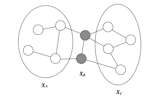
- If a set of observed variables forms a cut-set between two halves of the graph, then variables in one half are independent from ones in the other.
Cut-Set Variable Independencies
Markov Blanket
- The Markov blanket $U$ of a variable $X$ is the minimal set of nodes such that $X$ is independent from the rest of the graph if $U$ is observed. $$X \perp (\mathcal{X} - \{X\} - U) \mid U$$
- In an undirected graph, the Markov blanket is a node's neighborhood.
Conditional Random Fields - What are conditional random fields?
Definition
- A conditional random field is a Markov random field over variables $\mathcal{X} \cup \mathcal{Y}$ which specifies a conditional distribution:
$$
\begin{aligned}
P(y \mid x) &= \frac{1}{Z(x)} \prod_{c \in C} \phi_{c}(x_{c}, y_{c}) \\
Z(x) &= \sum_{y \in \mathcal{Y}} \prod_{c \in C} \phi_{c}(x_{c}, y_{c})
\end{aligned}
$$
- Where $x \in \mathcal{X}$ and $y \in \mathcal{Y}$ are VECTOR-VALUED variables.
- Where $Z(x)$ is the partition function.
- Important Note 1: A conditional random field results in an instantiation of a new Markov random field for each input $x$.
- Important Note 2: A conditional random field is useful for structured prediction in which the output labels are predicted considering the neighboring input samples.
Features
- Assume the factors $\phi_{c}(x_{c}, y_{c})$ are of the following form:
$$\phi_{c}(x_{c}, y_{c}) = \exp(w_{c}^{T} f_{c}(x_{c}, y_{c}))$$
- Where $f_{c}(x_{c}, y_{c})$ can be an arbitrary set of features describing the compatibility between $x_{c}$ and $y_{c}$.
- Where $w_{c}^{T}$ is the transposed weight matrix.
- Accordingly, $f_{c}(x_{c}, y_{c})$ allows arbitrarily complex features.
- e.g., $f(x, y_{i})$ are features that depend on the entirety of input samples $x$.
- e.g., $f(y_{i}, y_{i + 1})$ are features that depend on successive pairs of output labels $y$.
Conditonal Random Fields vs. Markov Random Fields - Why is a conditional random field a special case of Markov random fields?
- If we were to model $p(x, y)$ using a Markov random field, then we need to fit two probability distributions to the data: $p(y \mid x)$ and $p(x)$.
- Remember Baye's Rule: $p(x, y) = p(y \mid x) \cdot p(x)$
- However, if all we are interested in is predicting $y$ given $x$, then modeling $p(x)$ is expensive and unnecessary. $$\text{Prediction} \implies \text{CRF} > \text{MRF}$$
Factor Graphs - What is a factor graph? Why does a factor graph exist?
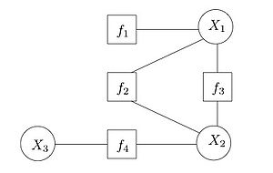
- A factor graph is a bipartite graph where one group is the variables in the distribution being modeled, and the other group is the factors defined on these variables.
- Edges Between Factors and Variables
- Side Note: A bipartite graph is a graph whose vertices are divided into two disjoint and independent sets.
- Set 1: Variables
- Set 2: Factors
- Important Note: Use a factor graph to identify what variables a factor depends on when computing probability distributions.
Inference 
- Problem: Given a probabilistic model, how do we obtain answers to relevant questions about the world?
- Marginal Inference: What is the probability of a given variable in our model after we sum everything else out?
$$p(y = 1) = \sum_{x_{1}} \sum_{x_{2}} \cdots \sum_{x_{n}} p(y = 1, x_{1}, x_{2}, ..., x_{n})$$
- e.g., What is the overall probability that an email is spam?
- Perspective: We desire to infer the general probability of some real-world phenomenon being observed.
- i.e., You care more about spam as a whole than specific instances of spam.
- Maximum A Posteriori: What is the most likely assignment of variables?
$$\max_{x_{1}, ..., x_{n}} p(y = 1, x_{1}, x_{2}, ..., x_{n})$$
- e.g., What is the set of words such that an email has the maximum probability of being spam?
- Perspective: We desire to infer the set of conditions that maximizes the probability of some real-world phenomenon being observed.
- i.e., You care more about identifying indicators of spam than detecting spam.
- Naive Complexity: NP-Hard (DIFFICULT PROBLEM)
- Marginal Inference: What is the probability of a given variable in our model after we sum everything else out?
$$p(y = 1) = \sum_{x_{1}} \sum_{x_{2}} \cdots \sum_{x_{n}} p(y = 1, x_{1}, x_{2}, ..., x_{n})$$
- Solution: Exact Inference Algorithms & Approximate Inference Algorithms
Vairable Elimination (Exact Inference Algorithm) 
Motivation - Why does the variable elimination algorithm exist?
- Let $x_{i}$ be a discrete random variable that takes $k$ possible values.
- Problem: Marginal Inference $$p(y = 1) = \sum_{x_{1}} \sum_{x_{2}} \cdots \sum_{x_{n}} p(y = 1, x_{1}, x_{2}, ..., x_{n})$$
- Naive Solution's Time Complexity (Exponential): $O(k^{n})$
- Variable Elimination Solution's Time Complexity (Non-Exponential): $O(n \cdot k^{M + 1})$
- See Below. $$\therefore \text{Variable Elimination Solution} \ll \text{Naive Solution}$$
Factors - How should a probabilistic graphical model express a probability distribution?
- Assumption: Probabilistic Graphical Models = Product of Factors $$p(x_{1}, ..., x_{n}) = \prod_{c \in C} \phi_{c}(x_{c})$$
- Representation: A factor can be represented as a multi-dimensional table with a cell for each assignment of $x_{c}$.
- Bayesian Networks: $\phi$ is Conditional Probability Distribution
- Markov Random Fields: $\phi$ is Potentials
Factor Product - What is the product operation?
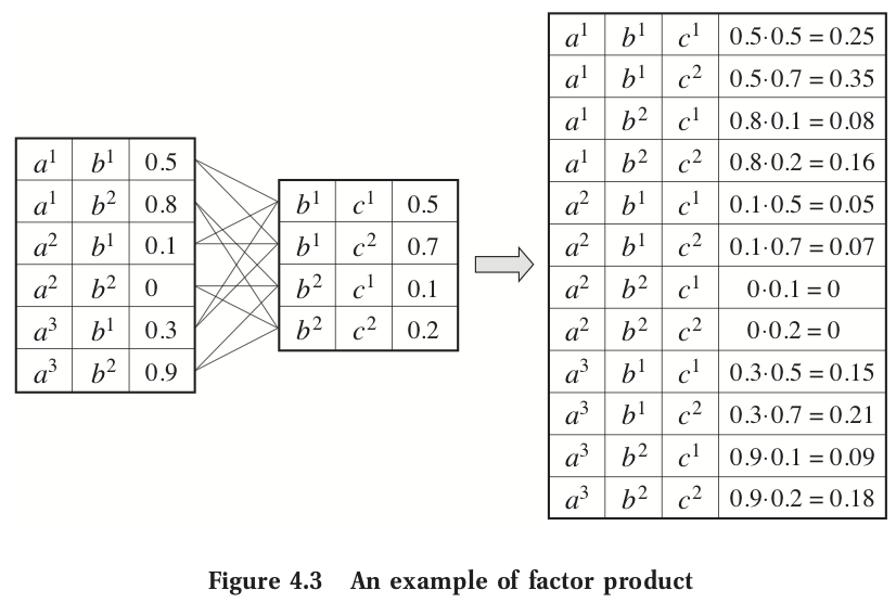
- Let $A$, $B$, and $C$ be three disjoint sets of variables.
- Let $\phi_{1}(A, B)$ and $\phi_{2}(B, C)$ be two factors.
- Let $\phi_{3}(A, B, C)$ be the factor product.
$$\phi_{3}(A, B, C) = \phi_{1}(A, B) \cdot \phi_{2}(B, C)$$
- Where the two factors are multiplied for common values of $B$.
Factor Marginalization - What is the marginalization operation?
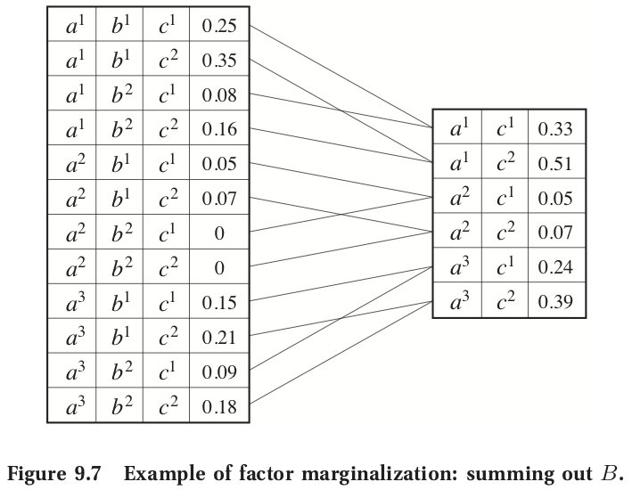
- Let $A$, and $B$ be two disjoint sets of variables.
- Let $\phi(A, B)$ be a factor.
- Let $\tau(A)$ be the factor marginalization of $B$ in $\phi$. $$\tau(A) = \sum_{B} \phi(A, B)$$
- Important Note: $\tau$ does not need necessarily correspond to a probability distribution.
Ordering - What is an ordering?
- An ordering $O$ is the sequence of variables by which they will be eliminated.
- Although any ordering can be used, different orderings may dramatically alter the running time of the variable elimination algorithm.
- Important Note: Finding Best Ordering = NP-Hard
Algorithm - How does the variable elimination algorithm work?
- For each variable $X_{i}$ (ordered according to $O$),
- Multiply all factors $\Phi_{i}$ containing $X_{i}$.
- Marginalize out $X_{i}$ to obtain a new factor $\tau$.
- Replace the factors $\Phi_{i}$ with $\tau$.
Time Complexity - What is the time complexity of variable elimination?
- Time Complexity: $O(n \cdot k^{M + 1})$
- Where $n$ is the number of variables.
- Where $M$ is the maximum number of dimensions of any factor $\tau$ formed during the elimination process.
Ordering Heuristics - How should you choose an ordering for variable elimination?
- Minimum Neighbors: Choose a variable with the fewest dependent variables.
- Minimum Weight: Choose variables to minimize the product of the cardinalities of its dependent variables.
- Minimum Fill: Choose vertices to minimize the size of the factor that will be added to the graph.
Evidence - How do you perform marginal inference given some evidence using variable elimination?
- Given a probability distribution $P(X, Y, E)$ with unobserved variables $X$, query variables $Y$, and observed evidence variables $E$, $P(Y \mid E = e)$ can be calculated using variable elimination. $$P(Y \mid E = e) = \frac{P(Y, E = e)}{P(E = e)}$$
Variable Elimination with Evidence
- Set every factor $\phi(X', Y', E')$ with values specified by $E = e$.
- Compute $P(Y, E = e)$ by performing variable elimination over $X$.
- Compute $P(E = e)$ by performing variable elimination over $Y$.
Example Problem 1 - Variable Elimination
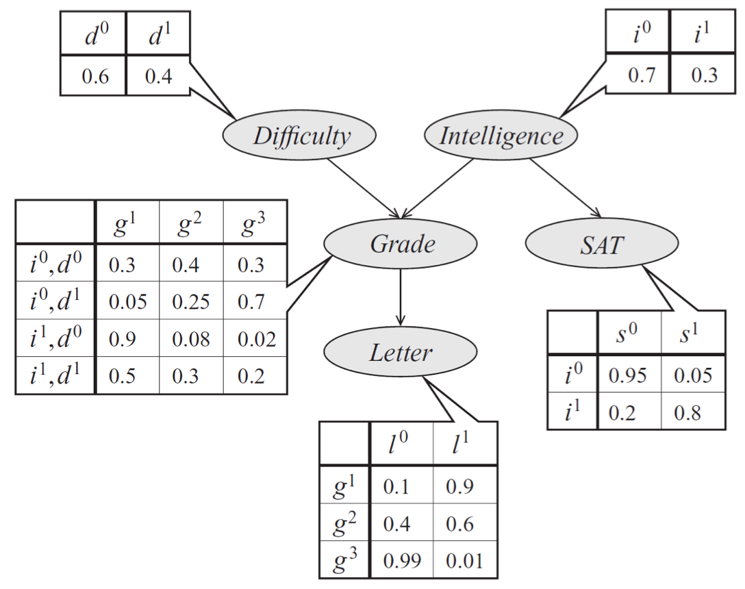
- A Bayesian network that models a student's grade on an exam:
- $g$ is a ternary variable of the student's grade.
- $d$ is a binary variable of the exam's difficulty.
- $i$ is a binary variable of the student's intelligence.
- $l$ is a binary variable of the quality of a reference letter from the professor who taught the course.
- $s$ is a binary variable of the student's SAT score. $$p(l, g, i, d, s) = p(l \mid g) \cdot p(s \mid i) \cdot p(i) \cdot p(g \mid i, d) \cdot p(d)$$
Question (Marginal Inference)
- What is the probability distribution of the quality of a reference letter from the professor who taught the course? $$p(l) = \sum_{g} \sum_{i} \sum_{d} \sum_{s} p(l, g, i, d, s)$$
Solution (Variable Elimination)
- Order the variables according to the topological sort of the Bayesian network. $$d, i, s, g$$
- Eliminate $d$ with a new factor $\tau_{1}$: $$ \begin{aligned} \tau_{1}(g, i) &= \sum_{d} p(g \mid i, d) \cdot p(d) \\ p(l, g, i, s) &= p(l \mid g) \cdot p(s \mid i) \cdot p(i) \cdot \tau_{1}(g, i) \end{aligned} $$
- Eliminate $i$ with a new factor $\tau_{2}$: $$ \begin{aligned} \tau_{2}(g, s) &= \sum_{i} p(s \mid i) \cdot p(i) \cdot \tau_{1}(g, i) \\ p(l, g, s) &= p(l \mid g) \cdot \tau_{2}(g, s) \end{aligned} $$
- Eliminate $s$ with a new factor $\tau_{3}$: $$ \begin{aligned} \tau_{3}(g) &= \sum_{s} \tau_{2}(g, s) \\ p(l, g) &= p(l \mid g) \cdot \tau_{3}(g) \end{aligned} $$
- Eliminate $g$ with a new factor $\tau_{4}$: $$ \begin{aligned} \tau_{4}(l) &= \sum_{g} p(l \mid g) \cdot \tau_{3}(g) \\ p(l) &= \tau_{4}(l) \end{aligned} $$
- Expanding $\tau_{i}$: $$p(l) = \sum_{g} p(l \mid g) \cdot \sum_{s} \sum_{i} p(s \mid i) \cdot p(i) \cdot \sum_{d} p(g \mid i, d) \cdot p(d)$$
Time Complexity
- Naive Solution: $O(k^{4})$
- Variable Elimination Solution: $O(4 \cdot k^{3})$
- Step 2. takes $O(k^{3})$ steps as the factor product $p(g \mid i, d) \cdot p(d)$ has a $3$-dimensional table representation, and the factor marginalization of $d$ can execute concurrently with the factor product.
- Step 3. takes $O(k^{3})$ steps as the factor product $p(s \mid i) \cdot p(i) \cdot \tau_{1}(g, i)$ has a $3$-dimensional table representation, and the factor marginalization of $i$ can execute concurrently with the factor product.
- Step 4. takes $O(k)$ steps for the factor marginalization of $s$.
- Step 5. takes $O(k^{2})$ steps as the factor product $p(l \mid g) \cdot \tau_{3}(g)$ has a $2$-dimensional table representation, and the factor marginalization of $g$ can execute concurrently with the factor product.
- As $O(k^{3})$ is the largest step, with $4$ steps, the time complexity is at most $O(4 \cdot k^{3})$.
- Thus, with $n = 4$ and $M = 2$, the time complexity is at most $O(n \cdot k^{M + 1}) = O(4 \cdot k^{3})$.
MAP Inference 
Overview - What is MAP inference?
- See Inference.
- Given a probabilistic graphical model $p(x_{1}, ..., x_{n}) = \prod_{c \in C} \phi_{c}(x_{c})$, MAP inference corresponds to the following optimization problem:
$$\max_{x} \log p(x) = \max_{x} \sum_{c \in C} \theta_{c}(x_{c}) - \log Z$$
- Where $\theta_{c}(x_{c}) = \log \phi_{c}(x_{c})$.
Derivation - Why is the MAP inference optmization problem expressed the way it is?
- All probabilistic graphical models (as BNs and CRFs are special cases of MRFs) have the following representation:
$$p(x) = \frac{1}{Z} \prod_{c \in C} \phi_{c}(x_{c})$$
- Where $Z$ is NP-Hard.
- MAP inference desires to infer the set of conditions that maximizes the probability of some real-world phenomenon being observed. $$\max_{x} p(x) = \max_{x} \frac{1}{Z} \prod_{c \in C} \phi_{c}(x_{c})$$
- As $Z$ is expensive to calculate, maximize $\log p(x)$ instead of $p(x)$. $$\max_{x} \log p(x) = \max_{x} \log \left[ \frac{1}{Z} \prod_{c \in C} \phi_{c}(x_{c}) \right]$$
- Simplify using logarithmic identities.
- $\log(x \times y) = \log(x) + \log(y)$
- $\log(x \div y) = \log(x) - \log(y)$ $$\max_{x} \log p(x) = \max_{x} \left[ \sum_{c} \log \phi_{c}(x_{c}) - \log Z \right]$$
- Simplify using maximum identities.
- $\max_{x}(x \pm 1) = \max_{x}(x) \pm 1$ $$\max_{x} \log p(x) = \max_{x} \sum_{c} \log \phi_{c}(x_{c}) - \log Z$$
- Let $\theta_{c}(x_{c}) = \log \phi_{c}(x_{c})$. $$\max_{x} \log p(x) = \max_{x} \sum_{c \in C} \theta_{c}(x_{c}) - \log Z$$
- As $\log Z$ is outside the scope of the maximization, if you desire to infer the set of conditions that maximizes the probability of some real-world phenomenon being observed, then solve the following optimization problem: $$\arg \max_{x} \log p(x) = \arg \max_{x} \sum_{c \in C} \theta_{c}(x_{c})$$
- Important Note 1: Without $Z$, this optimization problem suggests that MAP inference is computationally cheaper than marginal inference questions.
- Important Note 2: As maximization and summation both distribute over products, techniques used to solve marginal inference problems can be used to solve MAP inference problems.
Graph Cuts - How can MAP inference problems be solved using graph cuts?
- A graph cut of an undirected graph $G = (V, E)$ is a partition of $V$ into two disjoint sets $V_{s}$ and $V_{t}$.
- The min-cut problem is to find the partition $V_{s}, V_{t}$ that minimize the cost of the graph cut.
- The cost of a graph cut is the sum of the nonnegative costs of the edges that cross between the two partitions: $$\text{cost}(V_{s}, V_{t}) = \sum_{v_{1} \in V_{s}, v_{2} \in V_{t}} \text{cost}(v_{1}, v_{2})$$
- Time Complexity 1: $O(\lvert E \rvert \lvert V \rvert \log \lvert V \rvert)$
- Time Complexity 2: $O({\lvert V \rvert}^{3})$
- A MAP inference problem can be reduced into the min-cut problem in certain restricted cases of MRFs with binary variables.
Linear Programming - How can MAP inference problems be solved using linear programming?
- An approximate approach to computing the MAP values is to use Integer Linear Programming by introducing:
- An indicator variable per variable in the PGM.
- An indicator variable per edge/clique in the PGM.
- Constraints on consistent values in cliques.
Local Search - How can MAP inference problems be solved using local search?
- A heuristic solution that starts with an arbitrary assignment and performs modifications on the joint assignment that locally increase the probability.
Branch and Bound - How can MAP inference problems be solved using branch and bound?
- An exhaustive solution that searches over the space of assignments while pruning branches that can be provably shown not to contain a MAP assignment.
Simulated Annealing - How can MAP inference problems be solved using simulated annealing?
- A sampling solution that expresses a probability distribution with the following:
$$p_{t}(x) \propto \exp\left( \frac{1}{t} \sum_{c \in C} \theta_{c}(x_{c}) \right)$$
- Where $t$ is temperature.
- $t \to \infty$ $\implies$ $p_{t}$ approaches a continuous uniform distribution.
- $t \to 0$ $\implies$ $p_{t}$ approaches a continuous exponential distribution with a significant peak of $\arg \max_{x} \sum_{c \in C} \theta_{c}(x_{c})$.
- Where $t$ is temperature.
- As the peak is a MAP assignment, a sampling algorithm starting with a high temperature which gradually decreases can eventually find the peak, given a sufficiently slow cooling rate.
Sampling-Based Inference 
Motivation - Why does sampling-based inference algorithms exist?
- Exact Inference Algorithms: Slow/NP-Hard
- Approximate Inference Algorithms: Marginal Inference, MAP Inference, Expectations
Expectations $\mathbb{E}[f(X)]$ - Why do we want to estimate expectations of random variables?
- Abstractly, approximate inference algorithms want to estimate the probability of some real-world phenomenon.
- Mathematically, estimating a probability $p(x)$ is a SPECIALIZATION of estimating an expectation $\mathbb{E}_{x \sim p}[f(x)] = \sum_{x} f(x)p(x)$
- If $f(x) = \mathbb{I}_{\lvert x \rvert}$, where $\mathbb{I}_{\lvert x \rvert}$ is an indicator function for event $x$, $$\mathbb{E}_{x \sim p}[\mathbb{I}_{\lvert x \rvert}] = p(x)$$
Multinomial Sampling - How do you sample a discrete CPD?
- Let $p$ be a multinomial probability distribution with event values $\{x^{1}, ..., x^{k}\}$ and event probabilities $\{\theta_{1}, ..., \theta_{k}\}$.
- Generate a sample $s$ uniformly from the interval $[0, 1]$.
- Partition the interval into $k$ subintervals: $$[0, \theta_{1}), [\theta_{1}, \theta_{1} + \theta_{2}), ..., \left[ \sum_{j = 1}^{i - 1} \theta_{j}, \sum_{j = 1}^{i} \theta_{j} \right)$$
- If $s$ is in the $i$th interval, then the sampled value is $x^{i}$.
- Time Complexity: $O(\log k)$ - Using Binary Search
- Remember Baye's Rule: $p(y \mid x) = \frac{p(x, y)}{p(x)}$
- $p(x, y)$ is a multinomial probability distribution.
Forward Sampling - How do you sample a discrete Bayesian network?
- Let $G$ be a Bayesian network representing a probability distribution $p(x_{1}, ..., x_{n})$.
- Sample the variables in a topological order.
- Sample the successor variables by conditioning these node's CPDs to the values sampled by their ancestors.
- Repeat until all $n$ variables have been sampled.
- Time Complexity: $O(n)$
Monte-Carlo Integration/Estimation - How do you take a large number of samples to estimate expectations?
- Monte-Carlo $\approx$ Large Number of Samples
$$\mathbb{E}_{x \sim p}[f(x)] \approx I_{T} = \frac{1}{T} \sum_{t = 1}^{T} f(x^{t})$$
- Where $x^{1}, ..., x^{T}$ are i.i.d. samples drawn according to $p$. $$ \begin{aligned} \mathbb{E}_{x^{1}, ..., x^{T} \sim^{\text{i.i.d.}} p}[I_{T}] &= \mathbb{E}_{x \sim p}[f(x)] \\ \text{Var}_{x^{1}, ..., x^{T} \sim^{\text{i.i.d.}} p}[I_{T}] &= \frac{1}{T} \text{Var}_{x \sim p}[f(x)] \end{aligned} $$
- Where the Monte-Carlo estimate $I_T$
Implications - What is important about Monte-Carlo estimations?
- $I_{T}$ is an unbiased estimator for $\mathbb{E}_{x \sim p}[f(x)]$.
- Referencing the Weak Law of Large Numbers, if $T \to \infty$, then $I_{T} \to \mathbb{E}_{x \sim p}[f(x)]$.
Rejection Sampling - How does rejection sampling work?
- Compute a target probability distribution $p(x)$ by sampling a proposal probability distribution $q(x)$, rejecting samples inconsistent with $p(x)$, and applying the Monte-Carlo estimation.
- Examples: See Rejection Sampling
- Disadvantage: Ignores Many Samples
Importance Sampling - How does importance sampling work?
- Compute a target probability distribution $p(x)$ by sampling a proposal probability distribution $q(x)$, reweighing samples with $w(x) = \frac{p(x)}{q(x)}$, and applying the Monte-Carlo estimation.
$$
\begin{aligned}
\mathbb{E}_{x \sim p}[f(x)] &= \sum_{x} f(x)p(x) \\
&= \sum_{x} f(x)\frac{p(x)}{q(x)}q(x) \\
&= \mathbb{E}_{x \sim q}[f(x)w(x)] \\
&\approx \frac{1}{T} \sum_{t = 1}^{T} f(x^{t})w(x^{t})
\end{aligned}
$$
- Examples: See Importance Sampling
- Advantage: Uses All Samples
Normalized Importance Sampling - How does normalized importance sampling work?
- Let $p(x)$ be unknown.
- Let $\tilde{p}(x) = Z \cdot p(x)$ be known.
- The weight $w(x) = \frac{\tilde{p}(x)}{q(x)}$ is invalid for unnormalized importance sampling.
- The normalizing constant of the distribution $\tilde{p}(x)$ is the following: $$\mathbb{E}_{x \sim q}[w(x)] = \sum_{x} q(x)\frac{\tilde{p}(x)}{q(x)} = \sum_{x} \tilde{p}(x) = Z$$
- The normalized importance sampling estimator is the following: $$ \begin{aligned} \mathbb{E}_{x \sim p}[f(x)] &= \sum_{x} f(x)p(x) \\ &= \sum_{x} f(x)\frac{p(x)}{q(x)}q(x) \\ &= \frac{1}{Z} \sum_{x} f(x)\frac{\tilde{p}(x)}{q(x)}q(x) \\ &= \frac{1}{Z} \mathbb{E}_{x \sim q}[f(x)w(x)] \\ &= \frac{\mathbb{E}_{x \sim q}[f(x)w(x)]}{\mathbb{E}_{x \sim q}[w(x)]} \end{aligned} $$
Markov Chain - What is a Markov chain?
- Markov Chain: A sequence of random variables $S_{0}, S_{1}, S_{2}, ...$ with each random variable $S_{i} \in \{1, 2, ..., d\}$ taking one of $d$ possible values.
- Initial State: $P(S_{0})$
- Subsequent States: $P(S_{i} \mid S_{i - 1})$
- Markov Assumption: $S_{i}$ cannot depend directly on $S_{j}$ where $j < i - 1$.
Stationary Distribution - Why is it important for a stationary distribution to exist?
- Let $T_{ij} = P(S_{\text{new}} = i \mid S_{\text{prev}} = j)$ be a $d \times d$ transition probability matrix.
- If the initial state $S_{0}$ is drawn from a vector probabilities $p_{0}$, the probability $p_{t}$ of ending in EACH STATE after $t$ steps is the following:
$$p_{t} = T^{t} p_{0}$$
- Where $T^{t}$ is matrix exponentiation.
- Stationary Distribution: If it exists, the limit $\pi = \lim_{t \to \infty} p_{t}$.
- Important Note 1: A Markov chain whose states are joint assignments to the variables in a probabilistic graphical model $p$ has a stationary distribution equal to $p$.
Existence of Stationary Distribution
- Irreducibility: It is possible to get from any state $x$ to any other state $x'$ with probability $>0$ in a finite number of steps.
- Aperiodicity: It is possible to return to any state at any time, i.e. there exists an $n$ such that for all $i$ and all $n' \ge n$, $P(s_{n'} = i \mid s_{0} = i) > 0$.
- Important Note 2: An irreducible and aperiodic finite-state Markov chain has a stationary distribution.
Markov Chain Monte Carlo - How do you sample from a MCMC?
- Let $T$ be a transition operator specifying a Markov chain whose stationary distribution is $p$.
- Le $x_{0}$ be an initial assignment to the variables of $p$.
- Run the Markov chain from $x_{0}$ for $B$ burn-in steps.
- If $B$ is sufficiently large, $\pi \to p$.
- Run the Markov chain for $N$ sampling steps and collect all the states that it visits.
- The collection of states form samples from $p$.
Applications of Markov Chain Monte Carlo
- Use samples for Monte Carlo integration to estimate expectations.
- Use samples to perform marginal inference.
- Use the sample with the highest probability to perform MAP inference.
Gibbs Sampling - How do you construct a MCMC?
- Let $x_{1}, ..., x_{n}$ be an ordered set of variables.
- Let $x^{0} = (x_{1}^{0}, ..., x_{n}^{0})$ be a starting configuration.
- Repeat until convergence for $t = 1, 2, ...$,
- Set $x \gets x^{t - 1}$.
- For each variable $x_{i}$,
- Sample $x_{i}' \sim p(x_{i} \mid x_{-i})$.
- Where $x_{-i}$ is all variables in $x$ except $x_{i}$
- Update $x \gets (x_{1}, ..., x_{i}', ..., x_{n})$.
- Sample $x_{i}' \sim p(x_{i} \mid x_{-i})$.
- Set $x^{t} \gets x$
- Important Note 1: When $x_{i}$ is updated, its new value is immediately used for sampling other variables $x_{j}$.
- Important Note 2: Every iteration of $x^{t}$ is a new sample from $p$.
Learning 
- Problem: Given a dataset $D$ of $m$ i.i.d. samples from some underlying distribution $p^{\ast}$, how do you fit the best model, given a family of models $M$, to make useful predictions?
- Parameter Learning: Where the graph structure is known, and we want to estimate the factors.
- Structure Learning: Where we want to estimate the graph, i,e. determine from data how the variables depend on each other.
- Solution: Best Approximation of $p^{\ast}$
- Density Estimation: We are interested in the full distribution.
- Specific Prediction Tasks: We are using the distribution to make a prediction.
- e.g. Is this email spam or not?
- Structure or Knowledge Discovery: We are interested in the model itself.
- e.g. How do some genes interact with each other?
Maximum Likelihood Estimation 
Motivation - Why does maximum likelihood estimation exist?
- Goal: How do we approximate $p$ as close as possible to $p^{\ast}$?
- Approach: When the KL divergence between $p$ and $p^{\ast}$ is minimal, $p$ is as close as possible to $p^{\ast}$.
KL Divergence - What is KL divergence?
- KL Divergence: How different is one probability distribution from another probability distribution? $$KL(p^{\ast} \parallel p) = \sum_{x} p^{\ast}(x) \log \frac{p^{\ast}(x)}{p(x)} = -H(p^{\ast}) - \mathbb{E}_{x \sim p^{\ast}}[\log p(x)]$$
Minimal KL Divergence - When is KL divergence minimal?
- General Idea: Minimizing KL Divergence $\Longleftrightarrow$ Maximizing Likelihood $$\min KL(p^{\ast} \parallel p) \Longleftrightarrow \max \mathbb{E}_{x \sim p^{\ast}}[\log p(x)]$$
- Because $p^{\ast}$ is unknown, approximate the log-likelihood with the emperical log-likelihood using a Monte-Carlo estimate. $$\mathbb{E}_{x \sim p^{\ast}}[\log p(x)] \approx \frac{1}{\lvert D \rvert} \sum_{x \in D} \log p(x)$$
Maximum Likelihood Learning - How do you fit the best model using maximum likelihood learning?
- Given a family of models $M$, to fit the best model $p$, compute the following. $$\max_{p \in M} \mathbb{E}_{x \sim p^{\ast}}[\log p(x)] \approx \max_{p \in M} \frac{1}{\lvert D \rvert} \sum_{x \in D} \log p(x)$$
Definition - What is maximum likelihood estimation?
- Maximum Likelihood Estimation: Given a data set $D$, choose parameters $\hat{\theta}$ that satisfy the following.
$$\max_{\theta \in \Theta} L(\theta, D)$$
- i.e., Maximize the parameters $\theta$ to best fit the data set $D$.
Loss Function - What is a loss function?
- Loss Function ($L(x, p)$): A measure of the loss that a model distribution $p$ makes on a particular instance $x$.
- e.g., MLE Loss Function: $L(x, p) = -\log p(x)$
- Important Note: Assuming instances are sampled from some distribution $p^{\ast}$, to fit the best model, MINIMIZE the expected loss. $$\mathbb{E}_{x \sim p^{\ast}}[L(x, p)] \approx \frac{1}{\lvert D \rvert} \sum_{x \in D} L(x, p)$$
Likelihood Function - What is a likelihood function?
- Likelihood Function ($L(\theta, D)$): The probability of observing the i.i.d. samples $D$ for all permissible values of the parameters $\theta$.
Example - Likelihood Function
- Let $p(x)$ be a probability distribution where $x \in \{h, t\}$ such that $p(x = h) = \theta$ and $p(x = t) = 1 - \theta$.
- Let $D = \{h, h, t, h, t\}$ be observed i.i.d. samples.
- Accordingly, $p(x)$ models the outcome of a biased coin where parameter $\theta$ represents the probability of flipping heads and $1 - \theta$ represents the probability of flipping tails.
- Express the likelihood function as the following. $$L(\theta, D) = \theta \cdot \theta \cdot (1 - \theta) \cdot \theta \cdot (1 - \theta) = \theta^{3} \cdot (1 - \theta)^{2}$$
Maximum Likelihood Learning - How does maximum likelihood learning estimate the CPDs in Bayesian networks?
- Let $p(x) = \prod_{i = 1}^{n} \theta_{x_{i} \mid x_{pa(i)}}$ be a Bayesian network.
- Where $\theta_{x_{i} \mid x_{pa(i)}}$ are parameters (CPDs) with UNKNOWN VALUES.
- Let $D = \{x^{(1)}, x^{(2)}, ..., x^{(m)}\}$ be i.i.d. samples.
- Let $L(\theta, D) = \prod_{i = 1}^{n} \prod_{j = 1}^{m} \theta_{x_{i}^{j} \mid x_{pa(i)}^{j}}$ be the likelihood function.
- Log and collect like terms of the likelihood function. $$\log L(\theta, D) = \sum_{i = 1}^{n} \sum_{x_{pa(i)}} \sum_{x_{i}} \#(x_{i}, x_{pa(i)}) \cdot \log \theta_{x_{i} \mid x_{pa(i)}}$$
- Maximize the (log) likelihood function by decomposing it into separate maximizations for the local conditional distributions.
- Important Note: The maximum-likelihood estimates of the parameters (CPDs) have closed-form solutions. $$\theta_{x_{i} \mid x_{pa(i)}}^{\ast} = \frac{\#(x_{i}, x_{pa(i)})}{\#(x_{pa(i)})}$$
Bayesian Learning 
Motivation - What are some problems with maximum likelihood estimation?
- A maximum likelihood estimate does not change as more data is observed because it assumes that the only source of uncertainty is explained by the parameters that are being fitted.
- Problem 1: Cannot Improve Confidence
- Problem 2: Cannot Incorporate Prior Knowledge
Definitions - What are a prior and a posterior?
- Bayesian Learning: Explicitly model uncertainty over both variables $X$ and parameters $\theta$ by letting parameters be random variables.
- A prior is the earlier probability distribution of parameter $\theta$ BEFORE observing data $D$.
- A posterior is the later probability distribution of parameter $\theta$ AFTER observing data $D$. $$p(\theta \mid D) = \frac{p(D \mid \theta) p(\theta)}{p(D)} \propto p(D \mid \theta) p(\theta)$$ $$posterior \propto likelihood \times prior$$
- Important Note 1: Bayes' rule allows prior knowledge to be incorporated into a model's parameters.
- Important Note 2: Using Bayes' rule, the numerator is easy to calculate, but the denominator is difficult to calculate.
- Important Note 3: The expected value of the posterior $p(\theta \mid D)$ is the estimate of the parameter $\theta$ that causes $p$ to be as close as possible to $p^{\ast}$.
Conjugate Priors - What is a conjugate prior?
- A parametric family $\phi$ is conjugate for the likelihood $P(D \mid \theta)$ if: $$P(\theta) \in \phi \implies P(\theta \mid D) \in \phi$$
- Important Note: If the normalizing constant of $\phi$ is known, then the denominator in Bayes' rule is easy to calculate.
Beta Distribution - What is the Beta distribution?
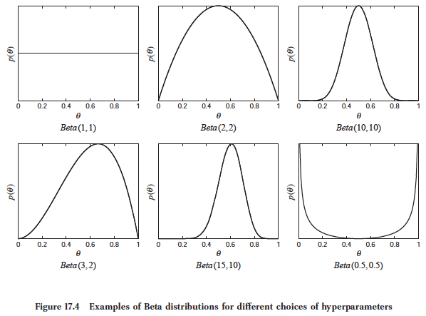
- A Beta distribution is parameterized by two hyperparameters $\alpha \in \mathbb{R}$, and $\beta \in \mathbb{R}$ with the following continuous probability distribution.
$$\theta \sim \text{Beta}(\alpha, \beta) \implies p(\theta) = \frac{\theta^{\alpha - 1} (1 - \theta)^{\beta - 1}}{B(\alpha, \beta)}$$
- Where $\theta \in (0, 1)$.
- Where the constant $\alpha$ intuitively corresponds to the number of SUCCESSES outcomes.
- Where the constant $\beta$ intuitively corresponds to the number of FAILURES outcomes.
- Where the constant $B(\alpha, \beta)$ is a normalizing constant defined by the following. $$B(\alpha, \beta) = \frac{\Gamma(\alpha) \Gamma(\beta)}{\Gamma(\alpha + \beta)}$$
- Where the Gamma function $\Gamma(x)$ is the continuous generalization of the factorial function defined by the following. $$\Gamma(x) = \int_{0}^{\infty} t^{x - 1} e^{-t} dt$$
- Expected Value: $$\mathbb{E}[X] = \frac{\alpha}{\alpha + \beta}$$
Conjugate Priors and Beta Distribution - How do you calculate a posterior with data observed from a binary process?
Think Coin Toss
- The beta distribution is the conjugate prior for the following probability distributions:
- Bernoulli: A discrete Bernoulli random variable, $X$, is the outcome from a single experiment from which this outcome is classified as either a success, $X = 1$ with probability $p$, or a failure, $X = 0$ with probability $1 - p$. $$ X \sim \text{Bernoulli}(p) \implies P(\{X = x\}) = \begin{cases} 1 - p & \text{if } x = 0 \\ p & \text{if } x = 1 \end{cases} $$
- Binomial: A discrete binomial random variable, $X$, is the number of successful outcomes from a sequence of $n$ independent experiments in which each experiment has an outcome classified as either a success with probability $p$ or a failure with probability $1 - p$ $$ X \sim \text{Binomial}(n, p) \implies P(\{X = x\}) = \binom{n}{x} p^x (1 - p)^{n - x} $$
- Geometric: A discrete geometric random variable, $X$, is the number of Bernoulli trials with probability $p$ needed to get one success. $$ X \sim \text{Geometric}(p) \implies P(\{X = x\}) = (1 - p)^{x - 1} p $$
- Negative Binomial: A discrete negative binomial random variable, $X$, is the number of successes in a sequence of independent and identically distributed Bernoulli trials before $r$ failures. $$ X \sim \text{Negative-Binomial}(r, p) \implies P(\{X = x\}) = \binom{x + r - 1}{x} p^x (1 - p)^r $$
- Important Note: To best fit a binary model with a probability distribution $p \approx p^{\ast}$, the beta distribution can be used by the following.
- Assign $\text{Beta}(\alpha, \beta)$ as a prior to $p$.
- Observe $n$ data points generated by a binary process with unknown, underlying $p^{\ast}$.
- If $X_{i} \sim \text{Bernoulli}(p^{\ast})$, then the posterior is $\text{Beta}(\alpha + \sum_{i = 1}^{n} x_{i}, \beta + n - \sum_{i = 1}^{n} x_{i})$.
- If $X_{i} \sim \text{Binomial}(N, p^{\ast})$, then the posterior is $\text{Beta}(\alpha + \sum_{i = 1}^{n} x_{i}, \beta + \sum_{i = 1}^{n} N_{i} - \sum_{i = 1}^{n} x_{i})$.
- If $X_{i} \sim \text{Geometric}(p^{\ast})$, then the posterior is $\text{Beta}(\alpha + n, \beta + \sum_{i = 1}^{n} x_{i} - n)$.
- If $X_{i} \sim \text{Negative-Binomial}(r, p^{\ast})$, then the posterior is $\text{Beta}(\alpha + \sum_{i = 1}^{n} x_{i}, \beta + rn)$.
Dirichlet Distribution (Multivariate Beta Distribution) - What is the Dirichlet distribution?
- A Dirichlet distribution is parameterized by the following hyperparameters $\pmb{\alpha} = (\alpha_{1}, ..., \alpha_{K}) \in \mathbb{R}^{K}$ with the following continuous probability distribution.
$$\theta \sim \text{Dirichlet}(\pmb{\alpha}) \implies p(\theta) = \frac{1}{B(\pmb{\alpha})} \prod_{i = 1}^{K} \theta_{i}^{\alpha_{i} - 1}$$
- Where $\theta_{i} \in (0, 1)$ and $\sum_{i = 1}^{K} \theta_{i} = 1$.
- Where the constant $\alpha_{i}$ intuitively corresponds to the number of outcomes for category $i$.
- Where the constant $B(\pmb{\alpha})$ is a normalizing constant defined by the following. $$B(\pmb{\alpha}) = \frac{\prod_{i = 1}^{K} \Gamma(\alpha_{i})}{\Gamma(\sum_{i = 1}^{K} \alpha_{i})}$$
- Where the Gamma function $\Gamma(x)$ is the continuous generalization of the factorial function defined by the following. $$\Gamma(x) = \int_{0}^{\infty} t^{x - 1} e^{-t} dt$$
- Expected Value: $$\mathbb{E}[X_{i}] = \frac{\alpha_{i}}{\sum_{k} \alpha_{k}}$$
Conjugate Priors and Dirichlet Distribution - How do you calculate a posterior with data observed from a categorical process?
Think $K$-Sided Dice Roll
- The Dirichlet distribution is the conjugate prior for the following probability distributions:
- Categorical (Generalized Bernoulli): A discrete categorical random variable, $X$, is the outcome from a single experiment from which this outcome is classified as one of $K$ categories with probability $p_{i} > 0$ and $\sum_{i = 1}^{K} p_{i} = 1$. $$ X \sim \text{Categorical}(\pmb{p}) \implies P(\{X = i\}) = p_{i} $$
- Multinomial (Generalized Binomial): A discrete multinomial random variable, $X$, is the number of outcomes from a sequence of $n$ independent experiments in which each experiment has an outcome classified as one of $K$ categories with probability $p_{i} > 0$ and $\sum_{i = 1}^{K} p_{i} = 1$. $$ X \sim \text{Multinomial}(n, \pmb{p}) \implies P(\{\pmb{X} = \pmb{x}\}) = \frac{n!}{x_{1}! ... x_{k}!} p_{1}^{x_{1}} ... p_{k}^{x_{k}} $$
- Important Note: To best fit a categorical model with a probability distribution $\pmb{p} \approx \pmb{p}^{\ast}$, the Dirichlet distribution can be used by the following.
- Assign $\text{Dirichlet}(\pmb{\alpha})$ as a prior to $\pmb{p}$.
- Observe $n$ data points generated by a categorical process with unknown, underlying $\pmb{p}^{\ast}$.
- If $X_{i} \sim \text{Categorical}(\pmb{p}^{\ast})$, then the posterior is $\text{Dirichlet}(\pmb{\alpha} + (c_{1}, ..., c_{K}))$.
- Where $c_{i}$ is the number of observations in category $i$.
- If $X_{i} \sim \text{Multinomial}(N, \pmb{p}^{\ast})$, then the posterior is $\text{Dirichlet}(\pmb{\alpha} + \sum_{i = 1}^{n} \pmb{x_{i}})$.
- If $X_{i} \sim \text{Categorical}(\pmb{p}^{\ast})$, then the posterior is $\text{Dirichlet}(\pmb{\alpha} + (c_{1}, ..., c_{K}))$.
Gamma Distribution - What is the Gamma distribution?
- A Gamma distribution is parameterized by two hyperparameters $\alpha \in \mathbb{R}$, and $\beta \in \mathbb{R}$ with the following continuous probability distribution.
$$\theta \sim \text{Gamma}(\alpha, \beta) \implies p(\theta) = \frac{\beta^{\alpha}}{\Gamma(\alpha)} \theta^{\alpha - 1} e^{-\beta \theta}$$
- Where $\theta \in (0, \infty)$.
- Where the constants $\alpha$ and $\beta$ intuitively corresponds to $\alpha$ total occurrences in $\beta$ intervals.
- Where the Gamma function $\Gamma(x)$ is the continuous generalization of the factorial function defined by the following. $$\Gamma(x) = \int_{0}^{\infty} t^{x - 1} e^{-t} dt$$
- Expected Value: $$\mathbb{E}[X] = \frac{\alpha}{\beta}$$
Conjugate Priors and Gamma Distribution - How do you calculate a posterior with data observed from a Poisson point process?
Think Rate (Events/Second)
- The Gamma distribution is the conjugate prior for the following probability distributions:
- Poisson: A discrete Poisson random variable, $X$, is the number of events occuring in a fixed interval of time or at a fixed rate. $$ X \sim \text{Poisson}(\lambda) \implies P(\{X = x\}) = e^{-\lambda} \frac{\lambda^x}{x!} $$
- Exponential: A continuous exponential random variable, $X$, is the time between events in a Poisson point process. $$ X \sim \text{Exponential}(\lambda) \implies P(\{X = x\}) = \lambda e^{-\lambda x} $$
- Important Note: To best fit a Poisson point model with a probability distribution $p \approx p^{\ast}$, the Gamma distribution can be used by the following.
- Assign $\text{Gamma}(\alpha, \beta)$ as a prior to $p$.
- Observe $n$ data points generated by a Poisson point process with unknown, underlying $p^{\ast}$.
- If $X_{i} \sim \text{Poisson}(\lambda^{\ast})$, then the posterior is $\text{Gamma}(\alpha + \sum_{i = 1}^{n} x_{i}, \beta + n)$.
- If $X_{i} \sim \text{Exponential}(\lambda^{\ast})$, then the posterior is $\text{Gamma}(\alpha + n, \beta + \sum_{i = 1}^{n} x_{i})$.
Decision Making Under Uncertainty 
A/B Testing 
Definition - What is A/B Testing?
- A randomized experiment with two variants, $A$ and $B$, that determines which of the two variants is more effective with their respective cohorts at achieving successes in $n$ trials.
Bayesian Learning and A/B Testing - How do you determine which of $A$ and $B$ are better after observing $n_{A}$ and $n_{B}$ trials?
- Let $0 < p_{A} < 1$ be the unknown probability that $A$ is truly effective.
- Let $0 < p_{B} < 1$ be the unknown probability that $B$ is truly effective.
- Let $\delta = A - B$ be the measure whether $A$ is more effective than $B$.
- Let $\text{Beta}(1, 1)$ be the initial prior for $p_{A}$.
- Use different values for $\alpha$ and $\beta$ to inject a subjective prior belief about $p_{A}$.
- Let $\text{Beta}(1, 1)$ be the initial prior for $p_{B}$.
- Use different values for $\alpha$ and $\beta$ to inject a subjective prior belief about $p_{B}$.
- Observe $n_{A}$ data points generated by a Bernoulli process with unknown, underlying $p_{A}$.
- Observe $n_{B}$ data points generated by a Bernoulli process with unknown, underlying $p_{B}$.
- Update the posterior $p_{A}$ given $n_{A}$ using Bayesian learning.
- Update the posterior $p_{B}$ given $n_{B}$ using Bayesian learning.
- Approximate the joint distribution of $\delta$ using a MCMC constructed using MCMCs of posteriors $p_{A}$ and $p_{B}$.
- Count the number of samples greater than 0 for the probability that $A$ is better than $B$; i.e. the area under the curve after 0.
- Count the number of samples less than 0 for the probability that $A$ is worse than $B$; i.e. the area under the curve before 0.
Multi-Armed Bandits 
- See Reinforcement Learning: An Introduction
- Chapter 2: Multi-armed Bandits
Definition - What is the Multi-armed bandit problem?
- A fixed limited set of resources must be allocated between competing (alternative) actions in a way that maximizes their expected reward, when each action's properties are only partially known at the time of allocation, and may become better understood as time passes or by allocating resources to the action.
Exploration-Exploitation Tradeoff Dilemma - What is the exploration-exploitation tradeoff dilemma?
- Exploitation: If we have chosen an action that yields a pretty good reward, do we keep choosing it to maintain a pretty good reward?
- Exploration: Otherwise, do we choose other actions in hopes of finding an even-better action?
Learning Rule as Averaging - What is the standard form of learning rules?
$$ \begin{aligned} \text{New Estimate} \gets \text{Old Estimate} + \text{Step Size} \cdot \left[ \text{Target} - \text{Old Estimate} \right] \end{aligned} $$$\epsilon$-Greedy Bandits Algorithm - How do you choose actions using the $\epsilon$-greedy bandits algorithm?
- Let $A_{t}$ be the action chosen from $k$ possibilities at time step $t$.
- Let $R_{t}$ be the independent and identically distributed reward yielded by action $A_{t}$.
- Let $Q_{t}(a)$ be the expected reward from choosing action $a$ until time step $t$.
- Let $N_{t}(a)$ be the number of times action $a$ was chosen until time step $t$.
- Initialize $Q_{0}(a) \gets 0, \forall a \in \{1, ..., k\}$.
- Initialize $N_{0}(a) \gets 0, \forall a \in \{1, ..., k\}$.
- Repeat for $t = 0, 1, 2, ...$,
- Set $A_{t} \gets \max_{a} Q_{t}(a)$ with probability $1 - \epsilon$.
- Set $A_{t} \gets \text{random}(a)$ with probability $\epsilon$.
- Sample $R_{t} \gets \text{bandit}(A_{t})$.
- Update $N_{t + 1}(A_{t}) \gets N_{t}(A_{t}) + 1$.
- Update $Q_{t + 1}(A_{t}) \gets Q_{t}(A_{t}) + \frac{1}{N_{t}(A_{t})}[R_{t} - Q_{t}(A_{t})]$.
$\epsilon$-Greedy Action Selection - How does $\epsilon$-greedy action selection work?
$$ A_{t} \gets \begin{cases} \max_{a} Q_{t}(a) & \text{ with probability } 1 - \epsilon \\ \text{random}(a) & \text{ with probability } \epsilon \end{cases} $$- Balances exploration and exploitation by choosing randomly a small fraction of the time.
- Problem: Indiscriminately, with no preference for those that are nearly greedy or particularly uncertain, selects non-greedy actions.
Upper-Confidence-Bound Action Selection - How does upper-confidence-bound action selection work?
$$ A_{t} \gets \max_{a} \left[ Q_{t}(a) + c \cdot \sqrt{\frac{\log t}{N_{t}(a)}} \right] $$- Balances exploration and exploitation by choosing deterministically but achieving exploration by subtly favoring at each step the actions that have so far received fewer samples.
- $\sqrt{\frac{\log t}{N_{t}(a)}}$ is a measure of the uncertainty or variance in the estimate of $a$’s value.
- $c > 0$ determines the confidence level by controlling the degree of exploration.
- $\log t$ increases the uncertainty in the estimate of $a$’s value as $a$ is exploited less.
- $N_{t}(a)$ decreases the uncertainty in the estimate of $a$’s value as $a$ is exploited more.
- Solution for $\epsilon$-Greedy Action Selection's Problem: As $\log t$'s increases get smaller over time, but are unbounded; all actions will eventually be selected, but actions with lower value estimates or that have already been selected frequently, will be selected with decreasing frequency over time.
Thompson Sampling Bandits Algorithm - How do you choose actions using the Thompson sampling bandits algorithm?
- Let $A_{t}$ be the action chosen from $k$ possibilities at time step $t$.
- Let $R_{t}$ be the independent and identically distributed reward yielded by action $A_{t}$.
- Let $p_{t}(a)$ be the initially unknown probabilitites of the rewards yielded by choosing action $a$ until time step $t$.
- Repeat for $t = 0, 1, 2, ...$,
- Sample a random variable $X_{a}$ using $p_{t}(a)$ for each $a \in \{1, ..., k\}$.
- Set $A_{t} \gets \max_{a} X_{a}$.
- Sample $R_{t} \gets \text{bandit}(A_{t})$.
- Update $p_{t + 1}(A_{t} \mid R_{t}) \propto p_{t}(R_{t} \mid A_{t}) p_{t}(A_{t})$.
- i.e., According to Bayesian learning.
Thompson Sampling Action Selection - How does Thompson sampling action selection work?
$$ \begin{aligned} X_{a} &\sim p_{t}(a) \\ A_{t} &\gets \max_{a} X_{a} \end{aligned} $$- Balances exploration and exploitation by sampling actions in proportion to the belief they are optimal.
- Solution for $\epsilon$-Greedy Action Selection's Problem: As TS selects actions according to SAMPLES from posterior distributions of the unknown probabilities that each respective action is optimal, TS explores to resolve uncertainty where there is a chance that resolution will help the agent identify the optimal action, but avoids probing where feedback would not be helpful.
Example: Thompson Sampling Intuition
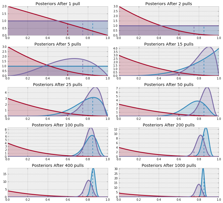
- The wider a posterior distribution, there is more uncertainty in probability that an action is optimal, so it still has the chance of generating the best sample at time $t$ which leads to further exploration to reduce uncertainty.
- The narrower a posterior distribution, there is less uncertainty in probability that an action is optimal, so either its action will be exploited more (if more certainty in its optimality) or explored less (if more certainty in its sub-optimality).
Upper-Confidence-Bounds and Thompson Sampling
- Both heuristics explore the actions that are currently predicted to be optimal, and they are optimistic about action if there is too little information.
- Bayesian Optimization: Both optimize Bayesian regret and their bounds can be converted between each other.
Limitations of Thompson Sampling
- Problems Not Requiring Exploration: Some problems are better solved by a greedy algorithm.
- Problems Not Requiring Exploitation: Some problems do not need a balance between exploration and exploitation.
- Time Sensitivity: Some time-sensitive problems favor intensification of exploitation than a balance between exploration and exploitation.
- Problems Requiring Careful Assessment of Information Gain: Some problems require a more careful assessment of the information actions provide instead of favoring the most promising actions.
Markov Decision Processes 
Agent-Environment Interface - How does an agent interact with its environment?

- At discrete time steps $t = 0, 1, 2, 3, ...$,
- The agent observes the state from the environment, at step $t$: $S_{t} \in \mathcal{S}$.
- The agent produces an action upon the environment, at step $t$: $A_{t} \in \mathcal{A}(S_{t})$.
- The agent gets a resulting reward from the environment: $R_{t + 1} \in \mathcal{R} \subset \mathbb{R}$.
- The environment transitions into the next state as a result of the agent's action: $S_{t + 1} \in \mathcal{S}^{+}$.
Markov Property - What is the Markov property?
- A state $S_{t}$ is Markov if and only if, $$\mathbb{P}[S_{t + 1} \mid S_t] = \mathbb{P}[S_{t + 1} \mid S_{1}, ..., S_{t}]$$
- Important Note: i.e., the future is independent of the past given the present.
Markov Process/Chain - What is a Markov process/chain?
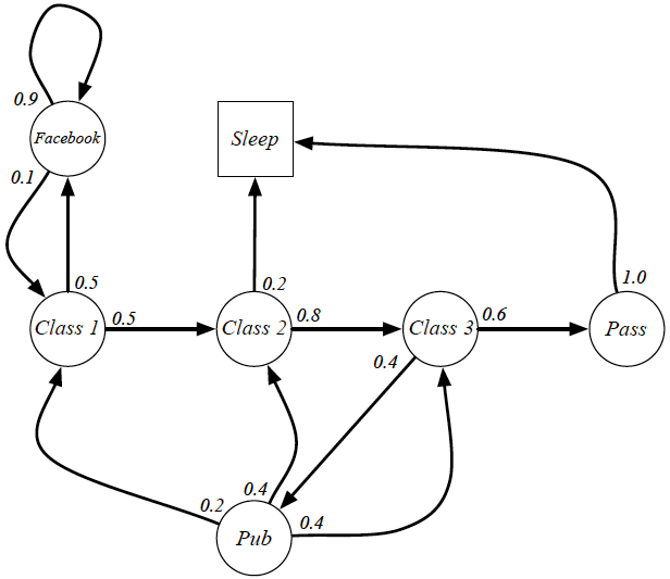
- A Markov process/chain is a tuple $\langle \mathcal{S}, \mathcal{P} \rangle$,
- $\mathcal{S}$ is a finite set of states.
- $\mathcal{P}$ is a state transition probability matrix, $\mathcal{P}_{ss'} = \mathbb{P}[S_{t + 1} = s' \mid S_{t} = s]$.
- Important Note: i.e., a memoryless random process.
Markov Reward Process - What is a Markov reward process?
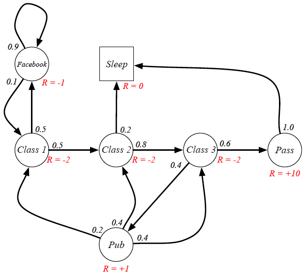
- A Markov reward process is a tuple $\langle \mathcal{S}, \mathcal{P}, \mathcal{R}, \gamma \rangle$
- $\mathcal{S}$ is a finite set of states.
- $\mathcal{P}$ is a state transition probability matrix, $\mathcal{P}_{ss'} = \mathbb{P}[S_{t + 1} = s' \mid S_{t} = s]$.
- $\mathcal{R}$ is a reward function, $\mathcal{R}_{s} = \mathbb{E}[R_{t + 1} \mid S_{t} = s]$.
- $\gamma \in [0, 1]$ is a discount factor.
Markov Decision Process - What is a Markov decision process?
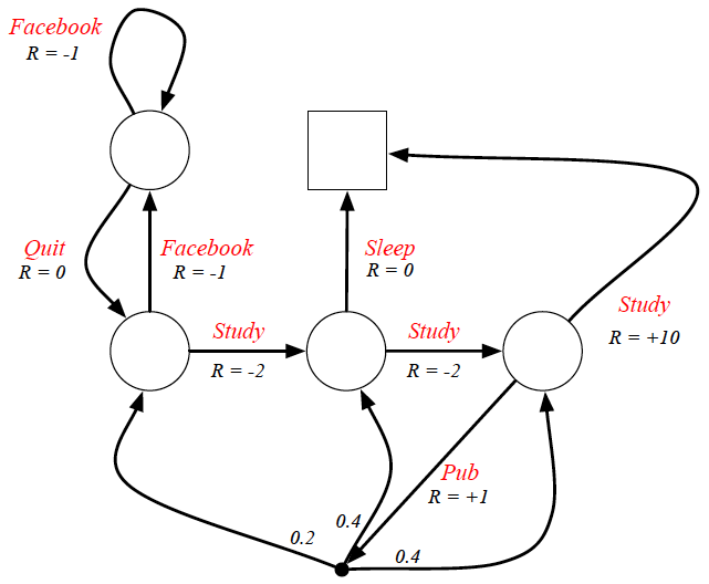
- A Markov decision process is a tuple $\langle \mathcal{S}, \mathcal{A}, \mathcal{P}, \mathcal{R}, \gamma \rangle$
- $\mathcal{S}$ is a finite set of states.
- $\mathcal{A}$ is a finite set of actions.
- $\mathcal{P}$ is a state transition probability matrix, $\mathcal{P}_{ss'}^{a} = \mathbb{P}[S_{t + 1} = s' \mid S_{t} = s, A_{t} = a]$.
- $\mathcal{R}$ is a reward function, $\mathcal{R}_{s}^{a} = \mathbb{E}[R_{t + 1} \mid S_{t} = s, A_{t} = a]$.
- $\gamma \in [0, 1]$ is a discount factor.
- Important Note: A majority of reinforcement learning problems can be formalized as MDPs.
Policy - What is a policy?
- A policy $\pi$ is a distribution over actions given states, $$\pi(a \mid s) = \mathbb{P}[A_{t} = a \mid S_{t} = s]$$
- Important Note 1: A policy fully defines the behavior of an agent.
- Important Note 2: Reinforcement learning methods specify how an agent changes its policy according to history.
Return - What is a return?
- The return $G_{t}$ is some measure of reward from time-step $t$. $$G_{t} = R_{t + 1} + \gamma \cdot R_{t + 2} + ... = \sum_{k = 0}^{\infty} \gamma^{k} R_{t + k + 1}$$
- Important Note: Reinforcement learning methods seek to maximize the expected return $\mathbb{E}[G_{t}]$, on each time-step $t$.
Variations of Reward
- Total Reward: The sum of all future rewards for episodic tasks.
- $\gamma = 1$.
- $R_{t} = 0, \forall t > T$, where $T$ is the terminal time-step.
- Discounted Reward: The sum of all future discounted rewards for continuous tasks.
- $\gamma \to 0$ implies shortsighted rewards.
- $\gamma \to 1$ implies farsighted rewards.
- Typically, $\gamma = 0.9$.
- Important Note: A discount factor avoids infinite returns in cyclic Markov processes.
Value Functions - What are the 4 value functions?
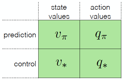
- The state-value function $v_{\pi}(s)$ is the expected return starting from state $s$, and then following policy $\pi$. $$v_{\pi}(s) = \mathbb{E}_{\pi}[G_{t} \mid S_{t} = s]$$
- The action-value function $q_{\pi}(s, a)$ is the expected return starting from state $s$, taking action $a$, and then following policy $\pi$. $$q_{\pi}(s, a) = \mathbb{E}_{\pi}[G_{t} \mid S_{t} = s, A_{t} = a]$$
- The optimal state-value function $v_{\ast}(s)$ is the maximum value function over all policies. $$v_{\ast}(s) = \max_{\pi} v_{\pi}(s)$$
- The optimal action-value function $q_{\ast}(s, a)$ is the maximum action-value function over all policies. $$q_{\ast}(s, a) = \max_{\pi} q_{\pi}(s, a)$$
- Important Note 1: The optimal value function specifies the best possible performance in the MDP.
- Important Note 2: A MDP is solved when the optimal value function is known.
Optimal Policy - What is an optimal policy?
- FOR ANY MDP,
- There exists an optimal policy $\pi_{\ast}$ that is better than or equal to all other policies, $\pi_{\ast} \ge \pi, \forall \pi$. $$\pi \ge \pi' \text{ if } v_{\pi}(s) \ge v_{\pi'}(s), \forall s$$
- All optimal policies achieve the same optimal value function, $v_{\pi_{\ast}}(s) = v_{\ast}(s)$.
- All optimal policies achieve the same optimal action-value function, $q_{\pi_{\ast}}(s, a) = q_{\ast}(s, a)$.
Finding a Deterministic Optimal Policy
$$ \pi_{\ast}(a \mid s) = \begin{cases} 1 &\text{ if } a = \max_{a \in \mathcal{A}} q_{\ast}(s, a)\\ 0 &\text{ otherwise} \end{cases} $$- Important Note: The optimal policy $\pi_{\ast}$ is greedy with respect to $q_{\ast}$ or $v_{\ast}$.
i.e., Deterministic Decision Making Under Uncertainty
Bellman Equation - What are the Bellman equations for the 4 value functions?
State-Value Function
$$ \begin{aligned} v_{\pi}(s) &= \mathbb{E}_{\pi}[G_{t} \mid S_{t} = s]\\ &= \mathbb{E}_{\pi}[R_{t + 1} + \gamma \cdot v_{\pi}(S_{t + 1}) \mid S_{t} = s]\\ &= \sum_{a \in \mathcal{A}} \pi(a \mid s) q_{\pi}(s, a)\\ &= \sum_{a \in \mathcal{A}} \pi(a \mid s) \left( \mathcal{R}_{s}^{a} + \gamma \sum_{s' \in \mathcal{S}} \mathcal{P}_{ss'}^{a} v_{\pi}(s') \right)\\ v_{\pi}(s) &= \sum_{a} \pi(a \mid s) \left[ \sum_{s', r} p(s', r \mid s, a) \left[ r + \gamma \cdot v_{\pi}(s') \right] \right] \end{aligned} $$Action-Value Function
$$ \begin{aligned} q_{\pi}(s, a) &= \mathbb{E}_{\pi}[G_{t} \mid S_{t} = s, A_{t} = a]\\ &= \mathbb{E}_{\pi}[R_{t + 1} + \gamma \cdot q_{\pi}(S_{t + 1}, A_{t + 1}) \mid S_{t} = s, A_{t} = a]\\ &= \mathcal{R}_{s}^{a} + \gamma \sum_{s' \in \mathcal{S}} \mathcal{P}_{ss'}^{a} v_{\pi}(s')\\ &= \mathcal{R}_{s}^{a} + \gamma \sum_{s' \in \mathcal{S}} \mathcal{P}_{ss'}^{a} \left( \sum_{a' \in \mathcal{A}} \pi(a' \mid s') q_{\pi}(s', a') \right)\\ q_{\pi}(s, a) &= \sum_{s', r} p(s', r \mid s, a) \left[ r + \gamma \cdot v_{\pi}(s') \right] \end{aligned} $$Optimal State-Value Function
$$ \begin{aligned} v_{\ast}(s) &= \max_{a} q_{\ast}(s, a)\\ &= \max_{a} \left( \mathcal{R}_{s}^{a} + \gamma \sum_{s' \in \mathcal{S}} \mathcal{P}_{ss'}^{a} v_{\ast}(s') \right)\\ v_{\ast}(s) &= \max_{a} \sum_{s', r} p(s', r \mid s, a) \left[ r + \gamma \cdot v_{\ast}(s') \right] \end{aligned} $$Optimal Action-Value Function
$$ \begin{aligned} q_{\ast}(s, a) &= \mathcal{R}_{s}^{a} + \gamma \sum_{s' \in \mathcal{S}} \mathcal{P}_{ss'}^{a} v_{\ast}(s') \\ &= \mathcal{R}_{s}^{a} + \gamma \sum_{s' \in \mathcal{S}} \mathcal{P}_{ss'}^{a} \left( \max_{a'} q_{\ast}(s', a') \right)\\ q_{\ast}(s, a) &= \sum_{s', r} p(s', r \mid s, a) \left[ r + \gamma \cdot \max_{a'} q_{\ast}(s', a') \right] \end{aligned} $$Reinforcement Learning 
Dynamic Programming 
Motivation - Why do you use dynamic programming to solve MDPs?
- MDPs have optimal substructure and overlapping subproblems in the recursive decomposition of Bellman equations.
- Appropriately, dynamic programming is used for planning in a MDP to predict and to control.
- Prediction: Given a MDP $\langle \mathcal{S}, \mathcal{A}, \mathcal{P}, \mathcal{R}, \gamma \rangle$ and a policy $\pi$, output a value function $v_{\pi}$.
- Control: Given a MDP $\langle \mathcal{S}, \mathcal{A}, \mathcal{P}, \mathcal{R}, \gamma \rangle$, output the optimal value function $v_{\ast}$ and the optimal policy $\pi_{\ast}$.
- Caveats 1: Requires Full Knowledge of MDP.
- Caveats 2: Polynomial Time, Yet Astronomically Large Number of States.
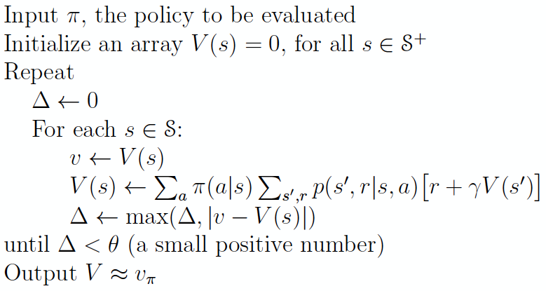
Policy Evaluation - How do you use dynamic programming to perform prediction?
Policy Improvement Theorem - How does policy iteration converge to the optimal policy?
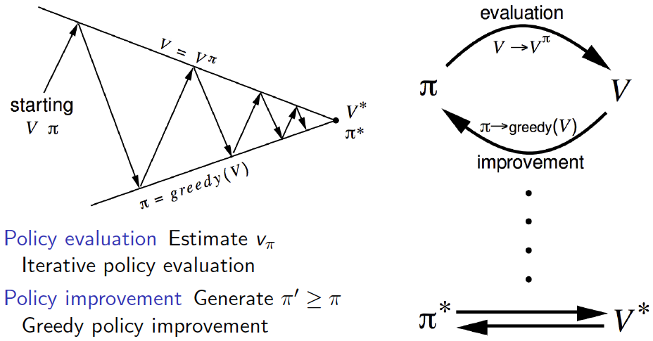
- Given a policy $\pi$,
- Evaluate the policy $\pi$, $$v_{\pi}(s) = \mathbb{E}_{\pi}[G_{t} \mid S_{t} = s]$$
- Improve the policy by acting greedily with respect to $v_{\pi}$. $$\pi' = \text{Greedy}(v_{\pi})$$
- The process of policy iteration has $\pi'$ converge to $\pi_{\ast}$ in a finite number of steps.
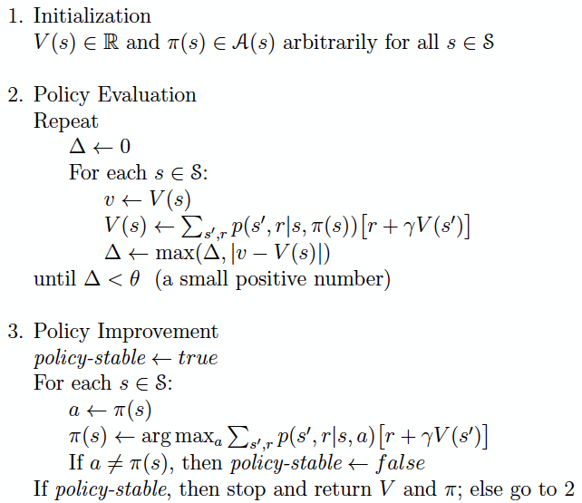
Policy Iteration - How do you use dynamic programming to perform control?
Backup Operations - What are sweeps and backups?

- A backup is a one-step lookahead, iterative application of the Bellman equation.
- A sweep is the iterative application of the backup operation to each state.
- Full Policy-Evaluation Backup: $$v_{k + 1}(s) = \sum_{a} \pi(a \mid s) \sum_{s', r} p(s', r \mid s, a) \left[ r + \gamma \cdot v_{k}(s') \right], \forall s \in S$$
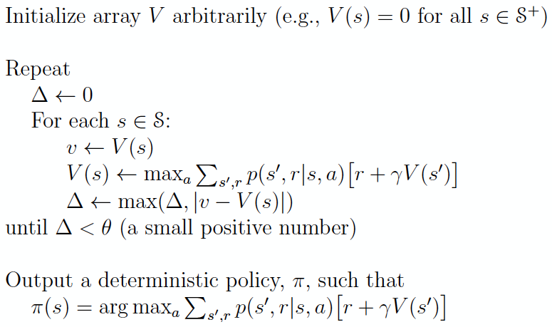
- Full Value-Iteration Backup: $$v_{k + 1}(s) = \max_{a} \sum_{s', r} p(s', r \mid s, a) \left[ r + \gamma \cdot v_{k}(s') \right], \forall s \in S$$
Value Iteration - How do you use dynamic programming to output a deterministic policy?
Backup Diagram - N/A
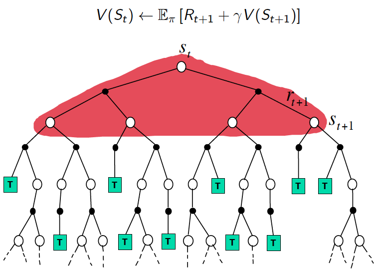
- Important Note: DP considers all the choices at each state, so it suffers a performance dilemma.
Monte-Carlo Reinforcement Learning 
Motivation - Why does Monte-Carlo reinforcement learning exist?
- Goal: How do you learn $v_{\pi}$ from episodes of experience under policy $\pi$?
- i.e. Model-Free Prediction
- Approach: Apply Monte-Carlo methods to learn $v_{\pi}$ as the empirical mean return instead of expected return.
- Advantages: No Bootstrapping, Model-Free, Time Complexity Independent from Number of States
- Disadvantages: All Episodes Must Terminate
First-Visit Monte-Carlo Policy Evaluation - How does first-visit Monte-Carlo policy evaluation perform prediction?
- To evaluate state $s$, the first time-step $t$ that state $s$ is visted in an episode,
- Increment counter $N(s) \gets N(s) + 1$.
- Increment total return $S(s) \gets S(s) + G_{t}$.
- Value is estimated by mean return $V(s) = \frac{S(s)}{N(s)}$.
- By the weak law of large numbers, $V(s) \to v_{\pi}(s)$ as $N(s) \to \infty$.
Every-Visit Monte-Carlo Policy Evaluation - How does every-visit Monte-Carlo policy evaluation perform prediction?
- To evaluate state $s$, the every time-step $t$ that state $s$ is visted in an episode,
- Increment counter $N(s) \gets N(s) + 1$.
- Increment total return $S(s) \gets S(s) + G_{t}$.
- Value is estimated by mean return $V(s) = \frac{S(s)}{N(s)}$.
- By the weak law of large numbers, $V(s) \to v_{\pi}(s)$ as $N(s) \to \infty$.
Backup Diagram - N/A
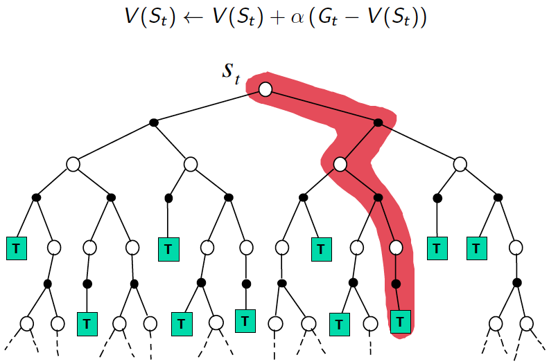
- Important Note: MC considers only one choice at each state, so it suffers from an explore/exploit dilemma.
Monte-Carlo Exploring Starts - How do you use Monte-Carlo Exploring Starts method to perform control?
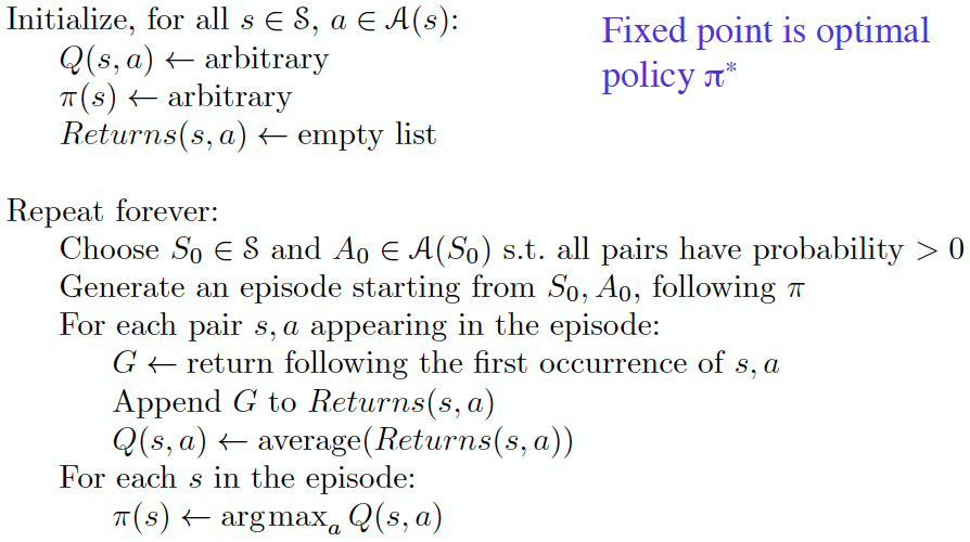
- Exploring Starts: Requires every state-action pair to have a non-zero probability of being the starting pair.
- Advantages: Asymptotically Converges
- Disadvantages: Restricts Modelling
On-Policy Monte-Carlo - How do you use On-Policy Monte-Carlo method to perform control?
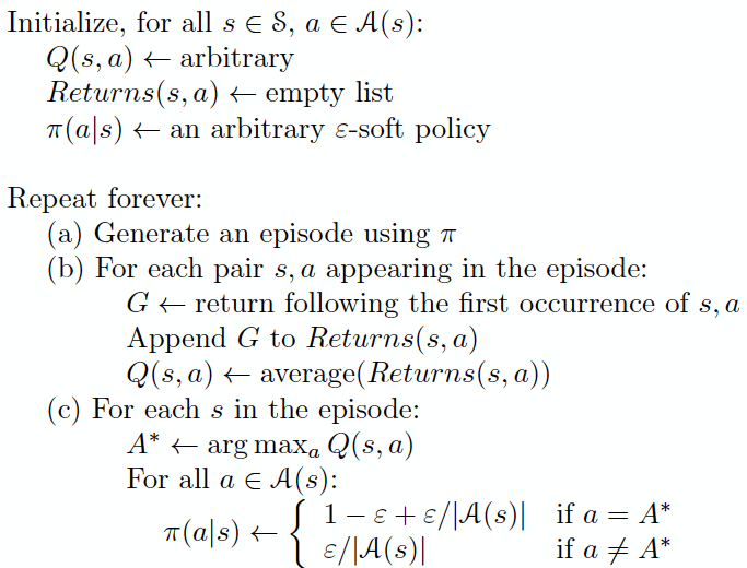
- On-Policy Learning: Learn about policy $\pi$ from experience sampled from $\pi$.
- i.e. Learn on the job.
- Soft Policy: Requires every state-action pair to have a non-zero probability.
- Advantages: Removes Exploring Starts
Off-Policy Monte Carlo - How do you use Off-Policy Monte-Carlo method to perform control?
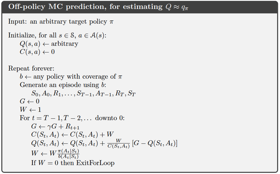
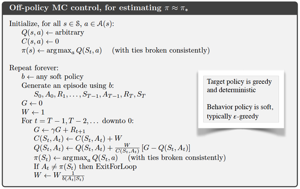
- Off-Policy Learning: Learn about policy $\pi$ from experience sampled from behavior policy $b$.
- i.e. Look over someone's shoulder.
- Behavior Policy: Requires $b$ generates behavior that covers, or includes, $\pi$.
$$b(a \mid s) > 0 \implies \pi(a \mid s) > 0, \forall a \in \mathcal{A}, s \in \mathcal{S}$$
- Question: How do you extract/emphasize $\pi$ from $b$?
- Answer: Use importance sampling.
- Importance Sampling: Weigh each return by the ratio of the probabilities of the trajectory under the two policies.
Importance Sampling - How do you calculate state-value function using importance sampling?
- Importance Sampling Ratio: A relative probability of the trajectory under the two policies. $$\rho_{t : T - 1} = \prod_{k = t}^{T - 1} \frac{\pi(A_{k} \mid S_{k})}{b(A_{k} \mid S_{k})}$$ $$\mathbb{E}\left[ \frac{\pi(A_{k} \mid S_{k})}{b(A_{k} \mid S_{k})} \right] = 1$$
Monte-Carlo Methods vs. Dynamic Programming - What are the advantages and disadvantages of Monte-Carlo methods?
Advantages
- Learn Directly from Interactions with Environment
- Does Not Require Full Models
- Does Not Require Learning About All States (No Bootstrapping)
- Less Harmed by Violating Markov Property
Disadvantages
- Requires Sufficient Exploration
- Requires Exploring Starts or Soft Policies
Temporal Difference Reinforcement Learning 
Motivation - Why does temporal difference reinforcement learning exist?
- Goal: How do you learn $v_{\pi}$ from incomplete episodes of experience under policy $\pi$?
- i.e. Model-Free Prediction
- Approach: Update an estimate of $v_{\pi}$ with an estimated return $G_{t}^{(n)}$ such as $G_{t}^{(1)} = R_{t + 1} + \gamma \cdot V(S_{t + 1})$.
- Advantages: Model-Free, Time Complexity Independent from Number of States, Incomplete Episodes
- Disadvantages: Bootstrapping
TD(0) Policy Evaluation - How does TD(0) policy evaluation perform prediction?
- Update value $V(S_{t})$ toward the estimated return $R_{t + 1} + \gamma \cdot V(S_{t + 1})$.
$$V(S_{t}) \gets V(S_{t}) + \alpha \left( R_{t + 1} + \gamma \cdot V(S_{t + 1}) - V(S_{t}) \right)$$
- Where $\alpha$ is a constant step-size.
- e.g., $\alpha = \frac{1}{N(s = S_{t})}$
- Where $R_{t + 1} + \gamma \cdot V(S_{t + 1})$ is the TD target.
- Where $\delta_{t} = R_{t + 1} + \gamma \cdot V(S_{t + 1}) - V(S_{t})$ is the TD error.
- Where $\alpha$ is a constant step-size.
Backup Diagram - N/A
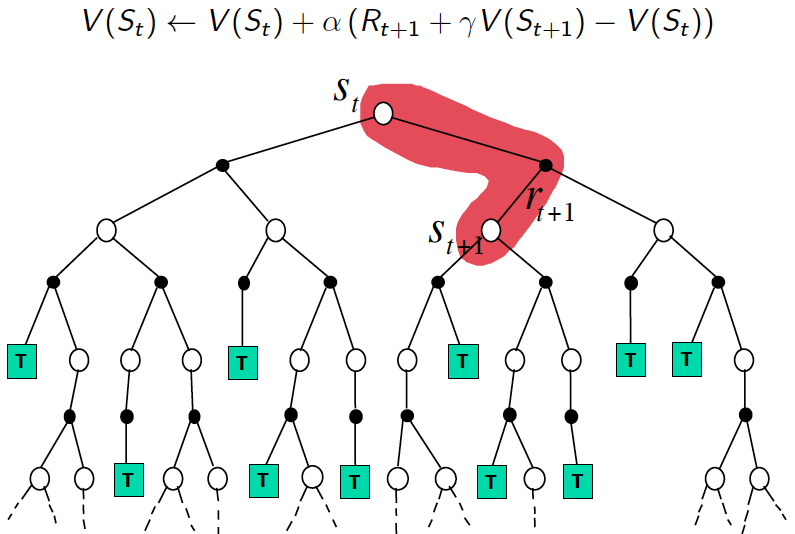
Temporal Difference vs. Monte-Carlo - What are the advantages and disadvantages of temporal difference methods?
Advantages
- Learn Without/Before Final Outcome
- Learn From Incomplete/Non-Terminating Sequences
- Low Variance
- Memory Efficienct
- Exploits Markov Property $\implies$ Less Error & Faster Convergence
Disadvantages
- Some Bias
- More Sensitive to Initial Parameters
SARSA - How is on-policy TD control achieved?
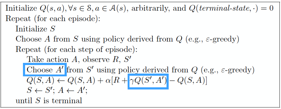
Q-Learning - How is off-policy TD control achieved?
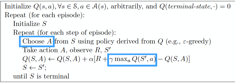
Expected SARSA - N/A
$$ \begin{aligned} Q(S_{t}, A_{t}) &= Q(S_{t}, A_{t}) + \alpha \left[ R_{t + 1} + \gamma \cdot \mathbb{E}[Q(S_{t + 1}, A_{t + 1}) \mid S_{t + 1}] - Q(S_{t}, A_{t}) \right] \\ Q(S_{t}, A_{t}) &= Q(S_{t}, A_{t}) + \alpha \left[ R_{t + 1} + \gamma \cdot \sum_{a} \pi(a \mid S_{t + 1})Q(S_{t + 1}, a) - Q(S_{t}, A_{t}) \right] \end{aligned} $$SARSA vs. Q-Learning - What are the similarities and differences between SARSA and Q-Learning?
SARSA
- On-Policy
- Chooses Action, Sees Result
- Update It's Value Function With Result
- Yes Guarantee Convergence
Q-Learning
- Off-Policy
- Chooses Action, Sees Result
- Update It's Value Function With Different Action
- No Guarantee Convergence
Multi-Step Reinforcement Learning 
Unified View of Reinforcement Learning - How are MC and TD methods of reinforcement learning related?
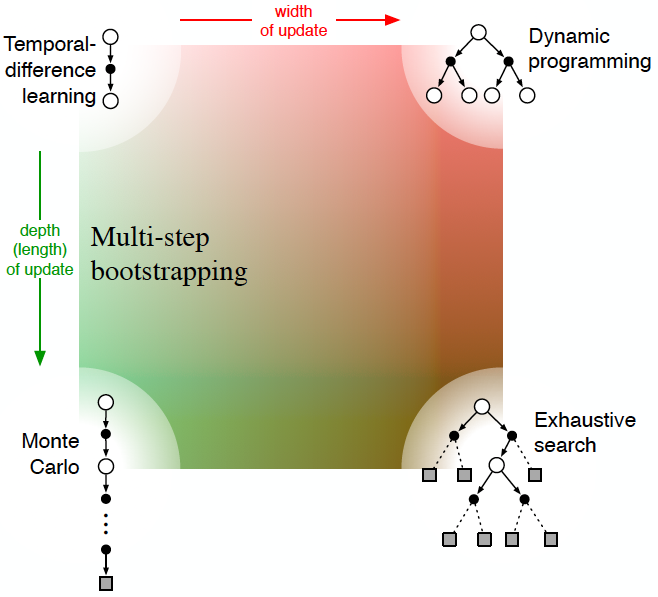
- MC: $n = \infty$-Steps of Predictions.
- $G_{t} = R_{t + 1} + \gamma \cdot R_{t + 2} + \gamma^{2} \cdot R_{t + 3} + ... + \gamma^{T - t - 1} \cdot R_{T}$
- TD: $n = 1$-Steps of Predictions.
- $G_{t : t + 1} = R_{t + 1} + \gamma \cdot V_{t}(S_{t + 1})$
$n$-Step TD - How do you use $n$-step TD to perform prediction?
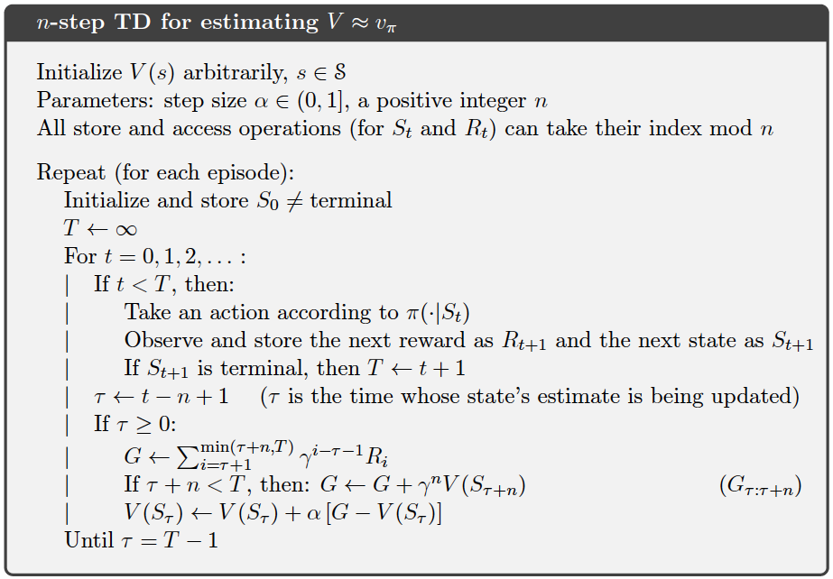
- $n$-Step Return (Forwards): $G_{t : t + n} = R_{t + 1} + \gamma \cdot R_{t + 2} + ... + \gamma^{n - 1} \cdot R_{t + n} + \gamma^{n} \cdot V_{t + n - 1}(S_{t + n})$
- $n$-Step TD (Backwards): $V_{t + n}(S_{t}) = V_{t + n - 1}(S_{t}) + \alpha \left[ G_{t : t + n} - V_{t + n - 1}(S_{t}) \right]$
- Important Note 1: The last $n$ states must be kept in memory.
- Important Note 2: Actual learning is delayed by $n$ steps.
On-Policy $n$-Step Control - How does the $n$-step method change on-policy control methods?
$n$-Step SARSA
$$ \begin{aligned} G_{t : t + n} &= R_{t + 1} + \gamma \cdot R_{t + 2} + ... + \gamma^{n - 1} \cdot R_{t + n} + \gamma^{n} \cdot Q_{t + n - 1}(S_{t + n}, A_{t + n}) \\ Q_{t + n}(S_{t}, A_{t}) &= Q_{t + n - 1}(S_{t}, A_{t}) + \alpha \left[ G_{t : t + n} - Q_{t + n - 1}(S_{t}, A_{t}) \right] \end{aligned} $$$n$-Step Expected SARSA
$$ \begin{aligned} G_{t : t + n} &= R_{t + 1} + \gamma \cdot R_{t + 2} + ... + \gamma^{n - 1} \cdot R_{t + n} + \gamma^{n} \cdot \mathbb{E}[Q_{t + n - 1}(S_{t + n}, A_{t + n}) \mid S_{t + n}] \\ G_{t : t + n} &= R_{t + 1} + \gamma \cdot R_{t + 2} + ... + \gamma^{n - 1} \cdot R_{t + n} + \gamma^{n} \cdot \sum_{a} \pi(a \mid S_{t + n})Q_{t + n - 1}(S_{t + n}, a) \\ Q_{t + n}(S_{t}, A_{t}) &= Q_{t + n - 1}(S_{t}, A_{t}) + \alpha \left[ G_{t : t + n} - Q_{t + n - 1}(S_{t}, A_{t}) \right] \end{aligned} $$Off-Policy $n$-Step Control - How does the $n$-step method change off-policy control methods?
Importance-Sampling Ratio
$$\rho_{t : h} = \prod_{k = t}^{\min(h, T - 1)} \frac{\pi(A_{k} \mid S_{k})}{b(A_{k} \mid S_{k})}$$Off-Policy $n$-Step TD
$V_{t + n}(S_{t}) = V_{t + n - 1}(S_{t}) + \alpha \rho_{t : t + n - 1} \left[ G_{t : t + n} - V_{t + n - 1}(S_{t}) \right]$
- Where $G_{t : t + n}$ is previously defined.
Off-Policy $n$-Step SARSA
$Q_{t + n}(S_{t}, A_{t}) = Q_{t + n - 1}(S_{t}, A_{t}) + \alpha \rho_{t + 1 : t + n - 1} \left[ G_{t : t + n} - Q_{t + n - 1}(S_{t}, A_{t}) \right]$
- Where $G_{t : t + n}$ is previously defined.
Off-Policy $n$-Step Expected SARSA
$Q_{t + n}(S_{t}, A_{t}) = Q_{t + n - 1}(S_{t}, A_{t}) + \alpha \rho_{t + 1 : t + n - 2} \left[ G_{t : t + n} - Q_{t + n - 1}(S_{t}, A_{t}) \right]$
- Where $G_{t : t + n}$ is previously defined.
$\lambda$-Return - What is $\lambda$-return?
- $\lambda$-Return: The return from averaging all $n$-step backups with $\lambda^{n - 1}$ weights. $$R_{t}^{\lambda} = (1 - \lambda) \sum_{n = 1}^{\infty} \lambda^{n - 1} R_{t}^{(n)}$$ $$\Delta V_{t}(s_t) = \alpha \left[ R_{t}^{\lambda} - V_{t}(s_{t}) \right]$$
- If $\lambda = 1$, TD$(1)$ is MC.
- If $\lambda = 0$, TD$(0)$ is TD$(0)$.
- If episodic, $\lambda$-return can be expressed by the following.
$$R_{t}^{\lambda} = (1 - \lambda) \sum_{n = 1}^{T - t - 1} \lambda^{n - 1} R_{t}^{(n)} + \lambda^{T - t - 1} R_{t}$$
- Where the first term represents the return until termination.
- Where the second term represents the return after termination.
Eligibility Trace - How do you use eligibility traces to compute TD$(\lambda)$?
- Eligibility Trace: A backward view mechanism for implementing TD$(\lambda)$ by decaying all traces by $\gamma \lambda$ and increment the trace for the current state by 1, and accumulating the trace. $$ e_{t}(s) = \begin{cases} \gamma \lambda e_{t - 1}(s) &\text{if } s \ne s_{t} \\ \gamma \lambda e_{t - 1}(s) + 1 &\text{if } s = s_{t} \end{cases} $$ $$\delta_{t} = r_{t + 1} + \gamma V_{t}(s_{t + 1}) - V_{t}(s_{t})$$ $$V_{t + 1}(s) = V_{t}(s) + \alpha \delta_{t} e_{t}(s)$$
- Important Note: Although TD$(1)$ is MC, TD$(1)$ executes incrementally and online.
Online Tabular TD$(\lambda)$ Algorithm - How does $\lambda$ extend TD for prediction?
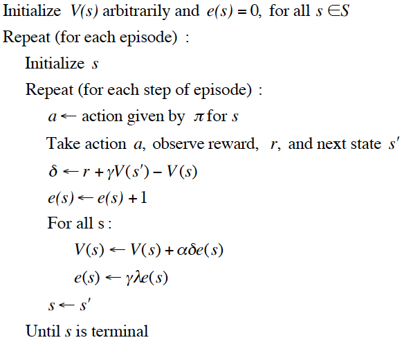
SARSA$(\lambda)$ Algorithm - How does $\lambda$ extend SARSA for on-policy control?
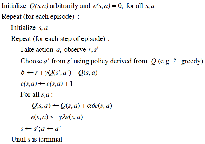
Watkin's Q$(\lambda)$ Algorithm - How does Watkin's algorithm achieve off-policy control?
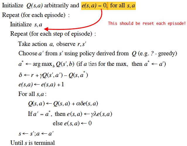
- Zero out eligibility trace after a non-greedy action.
- Take the maximum when backing up at the first non-greedy choice.
Peng's Q$(\lambda)$ Variant
- Never zero out eligibility trace after a non-greedy action.
- Take the maximum when backing up at the last non-greedy choice.
Naive Q$(\lambda)$ Variant
- Never zero out eligibility trace after a non-greedy action.
- Take the maximum when backing up at current action.
Value Function Approximation 
Motivation - Why does value function approximation exist?
- Goal: How do you represent a value function for a very large MDP whose states and/or actions cannot be all stored in memory inside a lookup table?
- Approach: Estimate the value function with function approximation, generalizing from known states to unknown states and updating parameter $\pmb{w}$ using MC or TD learning. $$ \begin{aligned} \hat{v}(s, \pmb{w}) &\approx v_{\pi}(s) \\ \hat{q}(s, a, \pmb{w}) &\approx q_{\pi}(s, a) \\ \end{aligned} $$
Differentiable Function Approximators
- Linear Combination of Features
- Neural Network
Gradient Descent - What is gradient descent?
- Let $J(\pmb{w})$ be a differentiable function of parameter vector $\pmb{w}$.
- The gradient of $J(\pmb{w})$ is the following. $$ \nabla_{\pmb{w}} J(\pmb{w}) = \left( \begin{array}{c} \frac{\partial J(\pmb{w})}{\partial \pmb{w}_{1}} \\ \vdots \\ \frac{\partial J(\pmb{w})}{\partial \pmb{w}_{n}} \end{array} \right) $$
- Gradient Descent: Adjust $\pmb{w}$ in the direction of the negative gradient to find a local minimum of $J(\pmb{w})$.
$$\Delta \pmb{w} = -\frac{1}{2} \alpha \nabla_{\pmb{w}} J(\pmb{w})$$
- Where $\alpha$ is a step-size parameter.
Stochastic Gradient Descent - How do you use stochastic gradient descent to approximate the value function?
- Find a parameter vector $\pmb{w}$ minimising mean-squared error between the approximate value function $\hat{v}(s, \pmb{w})$ and the true value function $v_{\pi}(s)$. $$J(\pmb{w}) = \mathbb{E}_{\pi}\left[ \left( v_{\pi}(S) - \hat{v}(S, \pmb{w}) \right)^{2} \right]$$
- A gradient descent finds a local minimum of $J(\pmb{w})$ such that the parameter vector $\pmb{w}$ has the approximate value function close to the true value function. $$\Delta \pmb{w} = \alpha \mathbb{E}_{\pi}\left[ \left( v_{\pi}(S) - \hat{v}(S, \pmb{w}) \right) \nabla_{\pmb{w}} \hat{v}(S, \pmb{w}) \right]$$
- Stochastic gradient descent samples the gradient. $$\Delta \pmb{w} = \alpha \left( v_{\pi}(S) - \hat{v}(S, \pmb{w}) \right) \nabla_{\pmb{w}} \hat{v}(S, \pmb{w})$$
Linear Value Function Approximation - What is one approximate value function representation?
Linear Combination of Features
$$\hat{v}(S, \pmb{w}) = \pmb{x}(S)^{T} \pmb{w} = \sum_{j = 1}^{n} \pmb{x}_{j}(S) \pmb{w}_{j}$$- Where $\pmb{x}$ is a feature vector constructed from the original perceptron, the Least-Mean-Square (LMS) algorithm, Support Vector Machines (SVMs), or etc....
Properties
- The objective function is quadratic in parameters $\pmb{w}$: $$J(\pmb{w}) = \mathbb{E}_{\pi}\left[ \left( v_{\pi}(S) - \pmb{x}(S)^{T} \pmb{w} \right)^{2} \right]$$
- The stochastic gradient descent converges on the GLOBAL OPTIMUM.
- The update rule is simple: $$ \begin{aligned} \nabla_{\pmb{w}} \hat{v}(S, \pmb{w}) &= \pmb{x}(S) \\ \Delta \pmb{w} &= \alpha \left( v_{\pi}(S) - \hat{v}(S, \pmb{w}) \right) \pmb{x}(S) \\ \text{Update} &= \text{Step-Size} \times \text{Prediction Error} \times \text{Feature Value} \end{aligned} $$
Incremental Prediction Algorithms - How do you substitute the true value function $v_{\pi}(s)$ in linear value function approximation?
- For MC, the substitute is the return $G_{t}$. $$\Delta \pmb{w} = \alpha \left( G_{t} - \hat{v}(S_{t}, w) \right) \nabla_{\pmb{w}} \hat{v}(S_{t}, \pmb{w})$$
- For TD$(0)$, the substitute is the TD target $R_{t + 1} + \gamma \cdot \hat{v}(S_{t + 1}, \pmb{w})$. $$\Delta \pmb{w} = \alpha \left( R_{t + 1} + \gamma \cdot \hat{v}(S_{t + 1}, \pmb{w}) - \hat{v}(S_{t}, w) \right) \nabla_{\pmb{w}} \hat{v}(S_{t}, \pmb{w})$$
- For TD$(\lambda)$, the substitute is the $\lambda$-return $G_{t}^{\lambda}$. $$\Delta \pmb{w} = \alpha \left( G_{t}^{\lambda} - \hat{v}(S_{t}, w) \right) \nabla_{\pmb{w}} \hat{v}(S_{t}, \pmb{w})$$
Gradient MC - N/A

Gradient TD - N/A
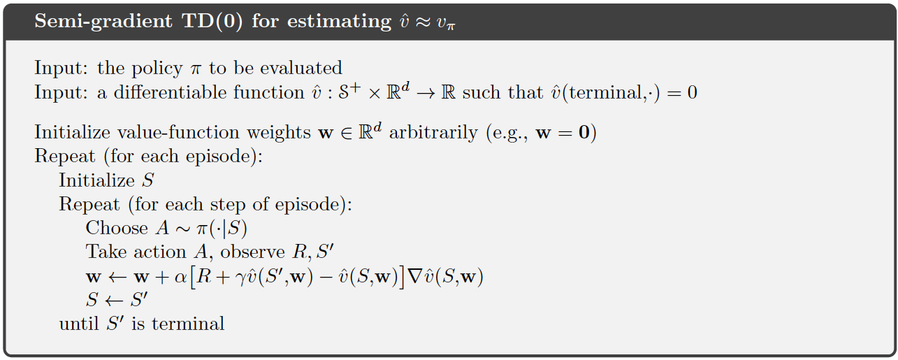
Gradient On-Policy Control - N/A
Learning Rule
$$\pmb{w}_{t + 1} = \pmb{w}_{t} + \alpha \left[ U_{t} - \hat{q}(S_{t}, A_{t}, \pmb{w}_{t}) \right] \nabla \hat{q}(S_{t}, A_{t}, \pmb{w}_{t})$$- MC: $U_{t} = G_{t}$
- SARSA: $U_{t} = R_{t + 1} + \gamma \cdot \hat{q}(S_{t + 1}, A_{t + 1}, \pmb{w}_{t})$
- Expected SARSA: $U_{t} = R_{t + 1} + \gamma \cdot \sum_{\alpha} \pi(\alpha \mid S_{t + 1}) \hat{q}(S_{t + 1}, \alpha, \pmb{w}_{t})$
Example
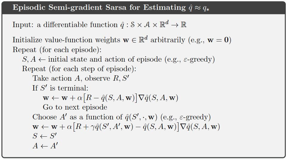
Deep Reinforcement Learning 
Introduction to Neural Networks 
Neural Networks - What is a neural network?
- A neural network connects many nonlinear (classically logistic/sigmoid) units together into a network to learn $f : \pmb{X} \to \pmb{Y}$.
- Where $f$ is a non-linear function.
- Where $\pmb{X}$ is a vector of continuous/discrete variables.
- Where $\pmb{Y}$ is a vector of continuous/discrete variables.
Three Layer Neural Network - What are the three layers in a basic neural network?
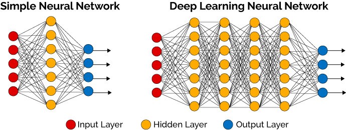
- Input Layer: Each input unit collects one feature/dimension of the vector data and passes it to the (first) hidden layer.
- Hidden Layer: Each hidden unit computes a weighted sum of all the units from the input later (or any previous layer) and passes it through a nonlinear activation function. $$y_{j} = f(net_{j})$$
- Output Layer: Each output unit computes a weighted sum of all the hidden units and passes it through a (possibly nonlinear) threshold function. $$z_{k} = f(net_{k})$$
Properties of Neural Networks - What are the properties of neural networks?
- Given a large enough layer of hidden units (or multiple layers), a NN can represent any function.
- Too few units, the network will be under-parameterized and will not be able to learn complex functions.
- Too many units, the network will be over-parameterized and will not be forced to learn a generlizable model.
- Connections between the units of all layers can be forward, backward, or both.
- Each unit can be fully or partially connected.
- Each unit has an activation function and a set of weighted connections.
Nonlinear Activation Function - What is a nonlinear activation function?
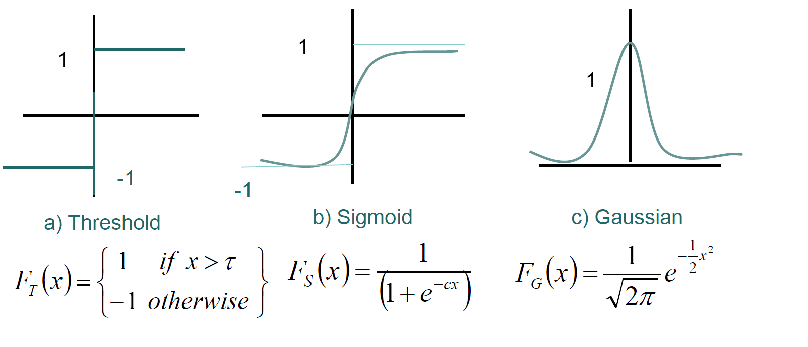
- A hidden unit emits an output that is a nonlinear activation function of its net activation.
$$y_{j} = f(net_{j}) = f \left( \sum_{i = 0}^{d} x_{i} w_{ji} \right)$$
- Where $i$ indexes the input units.
- Where $j$ indexes the hidden units.
- Where $w_{ji}$ denotes the synaptic weights.
- Outputs are thresholded through a nonlinear activation function.
- Rectified Linear Units (ReLU): The standard nonlinear activation function: $y_{j} = \max(0, net_{j})$.
- Easily distinguishes strong signals.
- Values are mostly zero.
- Derivative is mostly zero.
- Does not easily saturate compared to the sigmoid function.
Backpropagation Algorithm - How does the backpropagation algorithm iteratively compute the gradient to update network weights?
- Important Idea: Minimize the loss function (mean-squared errors) on training examples.
- Forward Propagation: Input the training data to the network and compute outputs.
- Compute output unit errors. $$\delta_{k}' = o_{k}' (1 - o_{k}') (y_{k}' - o_{k}')$$
- Compute hidden unit errors. $$\delta_{h}' = o_{h}' (1 - o_{h}') \sum_{k} w_{h,k} \delta_{k}'$$
- Update network weights. $$w_{i,j} = w_{i,j} + \Delta w_{i,j}' = w_{i,j} + \eta\delta_{j}'o_{i}'$$
- Where $y$ is the target output of a unit.
- Where $o$ is the actual output of a unit.
- Where $\eta$ is the training rate.
Deep Q-Networks (DQN) 
Motivation - What are the stability issues with naive deep Q-learning?
- A naive deep Q-learning approximates the action-value function by using a deep Q-network. However, it suffers from divergent and oscillating behavior.
- As data is sequential, the successive samples are correlated and not i.i.d., yet NNs require i.i.d. samples.
- Accordingly, the learned policy may oscillate with slight changes to Q-values.
- Finally, the scales of rewards and Q-values are unknown such that naive deep Q-learning gradients can be unstable when backpropagated.
Overview - What is a DQN?
- Use Experience Replay:
- Provides i.i.d. samples.
- Freeze Target Q-Network:
- Avoids oscillations.
- Clip Rewards / Normalize Network to Sensible Range:
- Stabilizes gradients.
Experience Replay - How does experience replay remove correlations to provide i.i.d. samples?
- Important Idea: To remove correlations, sample from the agent's own experience.
- Take action $a_{t}$ according to $\epsilon$-greedy policy.
- Store the transition $(s_{t}, a_{t}, r_{t + 1}, s_{t + 1})$ in the agent's replay memory $\mathcal{D}$.
- Sample a random mini-batch of transitions $(s, a, r, s')$ from $\mathcal{D}$.
- Optimise the mean squared error between the Q-network and the Q-learning targets. $$\mathcal{L}(\pmb{w}) = \mathbb{E}_{s, a, r, s' \sim \mathcal{D}}\left[ \left( r + \gamma \cdot \max_{a'} Q(s', a', \pmb{w}) - Q(s, a, \pmb{w}) \right)^{2} \right]$$
Frozen/Fixed Target Q-Network - How does freezing/fixing the target Q-network avoid oscillations?
- Important Idea: To avoid oscillations, freeze/fix parameters used in the Q-learning target.
- Compute the Q-learning targets with respect to the old, frozen/fixed parameters $\pmb{w}^{-}$. $$r + \gamma \cdot \max_{a'} Q(s', a', \pmb{w}^{-})$$
- Optimise the mean squared error between the Q-network and the Q-learning targets. $$\mathcal{L}(\pmb{w}) = \mathbb{E}_{s, a, r, s' \sim \mathcal{D}}\left[ \left( r + \gamma \cdot \max_{a'} Q(s', a', \pmb{w}^{-}) - Q(s, a, \pmb{w}) \right)^{2} \right]$$
- Periodically, update the frozen/fixed parameters: $\pmb{w}^{-} \gets \pmb{w}$.
Clip Rewards - How does clipping rewards stabilize gradients?
- Important Idea: To stabilize gradients, DQN clips rewards to a sensible range of $[-1, +1]$ such that Q-values can never become too large, ensuring that gradients are well-conditioned.
Policy Gradient 
Motivation - Why should you approximate policies versus action-values?
Advantages
- Better Convergence Properties
- High-Dimensional Action Spaces
- Continuous Action Spaces
- Stochastic Policies; e.g., Rock-Paper-Scissors
Disadvantages
- Typically, Converge Local Optimum vs. Global Optimum
- Typically, Inefficient Policy Evaluation
- Typically, High Variance Policy Evaluation
Policy Objective Functions - What policy objective functions can be used for a given type of environment?
- Goal: Given a policy $\pi(a \mid s, \pmb{\theta})$ with parameters $\pmb{\theta}$, find best $\pmb{\theta}$.
- Episodic Environments: Use Start Value. $$J_{1}(\pmb{\theta}) = V_{\pi}(s_{1}) = \mathbb{E}_{\pi}[v_{1}]$$
- Continuing Environments:
- Use Average Value. $$J_{avV}(\pmb{\theta}) = \sum_{s} d^{\pi}(s) V^{\pi}(s)$$
- Use Average Reward Per Time-Step. $$J_{avR}(\pmb{\theta}) = \sum_{s} d^{\pi}(s) \sum_{a} \pi(a \mid s, \pmb{\theta}) \mathcal{R}_{s}^{a}$$
- Where $d^{\pi}(s)$ is the stationary distribution of Markov chain for $\pi_{\pmb{\theta}}$.
Policy Gradient - How does policy gradient algorithms achieve policy based reinforcement learning?
- Important Idea: *Policy Based Reinforcement Learning = Finding $\pmb{\theta}$ That Maximises $J(\pmb{\theta})$.
- Policy gradient algorithms search for a local maximum in $J(\pmb{\theta})$ by ascending the gradient of the policy, with respect to parameters $\pmb{\theta}$.
$$\Delta\pmb{\theta} = \alpha \nabla_{\pmb{\theta}} J(\pmb{\theta})$$
- Where $\alpha$ is a step-size parameter.
Policy Gradient Theorem - How do you compute the policy gradient analytically?
Likelihood Ratios
$$ \begin{aligned} \nabla_{\pmb{\theta}} \pi(a \mid s, \pmb{\theta}) &= \pi(a \mid s, \pmb{\theta}) \frac{\nabla_{\pmb{\theta}} \pi(a \mid s, \pmb{\theta}) }{\pi(a \mid s, \pmb{\theta})} \\ &= \pi(a \mid s, \pmb{\theta}) \nabla_{\pmb{\theta}} \log \pi(a \mid s, \pmb{\theta}) \end{aligned} $$Softmax Policy (Popular)
- Weight actions using a linear combination of features $\phi(s, a)^{T} \pmb{\theta}$.
- Accordingly, the probability of an action is proportional to its exponentiated weight. $$\pi(a \mid s, \pmb{\theta}) \propto \exp(\phi(s, a)^{T} \pmb{\theta})$$
- Thus, the score function is the following. $$\nabla_{\pmb{\theta}} \log \pi(a \mid s, \pmb{\theta}) = \phi(s, a) - \mathbb{E}_{\pi}[\phi(s, \ast)]$$
Gaussian Policy (Continuous)
- Let the mean be a linear combination of state features $\mu(s) = \phi(s)^{T} \pmb{\theta}$.
- Let the variance be fixed/parameterised $\sigma^{2}$.
- Accordingly, an action is a Gaussian random variable. $$a \sim \mathcal{N}(\mu(s), \sigma^{2})$$
- Thus, the score function is the following. $$\nabla_{\pmb{\theta}} \log \pi(a \mid s, \pmb{\theta}) = \frac{(a - \mu(s)) \phi(s)}{\sigma^{2}}$$
Theorem
- For any differentiable policy $\pi(a \mid s, \pmb{\theta})$ and for any of the policy objective functions $J = J_{1}$, $J_{avR}$, or $\frac{1}{1 - \gamma} J_{avV}$, the policy gradient is the following. $$\nabla_{\pmb{\theta}} J(\pmb{\theta}) = \mathbb{E}_{\pi}\left[ \nabla_{\pmb{\theta}} \log \pi(a \mid s, \pmb{\theta}) \cdot Q^{\pi_{\pmb{\theta}}}(s, a) \right]$$
Monte-Carlo Policy Gradient (REINFORCE) - How does REINFORCE apply the policy gradient theorem?
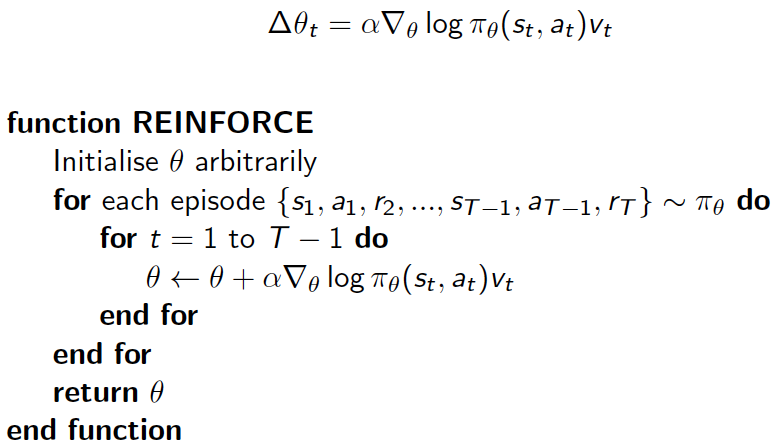
- It updates parameters using stochastic gradient ascent.
- It uses the return $v_{t}$ as an unbiased sample of $Q^{\pi_{\pmb{\theta}}}(s_{t}, a_{t})$.
- Problem: The Monte-Carlo policy gradient has high variance.
Actor-Critic Architecture - How does the actor-critic archiecture reduce variance in Monte-Carlo policy gradient algorithms?
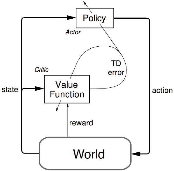
- Actor-critic methods consist of two models, which may optionally share parameters.
- Critic: Updates the action-value function parameters $\pmb{w}$.
- Actor: Updates policy parameters $\pmb{\theta}$, in the direction suggested by the critic.
Actor-Critic Formulas
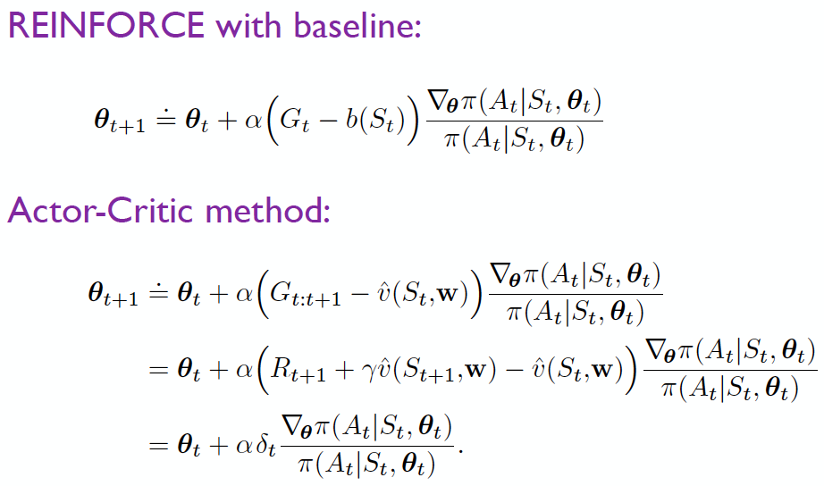
Actor-Critic Policy Gradient Algorithm - N/A
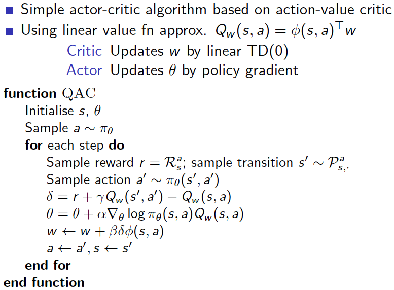
Actor-Critic Policy Gradient with Eligibility Traces Algorithm - N/A
